Go Back

Markov chain random field theory

This study was motivated first by attempts to solve the deficiencies of earlier multi-dimensional Markov chain spatial models (mainly the coupled Markov chain model, see "From the CMC model to the MCRF model") in order to model categorical spatial variables (e.g. soil types and layers), and then by attempts to develop a practical spatial/geo-statistical approach for categorical data estimation based on the single-chain Markov random-field idea. The generalized basic model for this approach (i.e., Markov chain random fields) conforms to a special, complex, spatial "Bayesian network" of spatial data points within a neighborhood without semantic causality. Therefore, it is different from conventional geo/spatial-statistics such as kriging and Markov random fields, and also different from conventional Bayesian networks, although the approach was mainly built on the knowledge in Makov chain theory, Bayesian theorem and conventional spatial/geo-statistics.

Markov chain random fields

A Markov chain random field (MCRF) is generally defined as a spatial Markov chain that moves or jumps in a space (one to multiple dimensions) with its local conditional probability distribution at any unobserved location to be conditional on nearest neighbors in different directions within a neighborhood (Li 2007a, Li and Zhang 2008). Such a single Markov chain traverses all of the unobserved locations in the space. This single-chain Markov random-field idea is the key idea for the MCRF theory. The interactions of the spatial Markov chain with nearest neighbors within a neighborhood centered on a specific unobserved location can be explained as a local sequential Bayesian updating process based on the evidence of nearest data (Li et al. 2013, 2015). Bayesian factorization of nearest spatial data within a neighborhood is a key idea for MCRFs. Therefore, the MCRF approach is in accordance with the Bayesian inference principle (Bayes 1763; Gelman et al. 1995; Jaffray 1992) and may represent a Bayesian spatial statistics approach. A MCRF can be 1D, 2D, 3D and even 4D (spatiotemporal). In 1D, it returns to a conventional or jumping 1D Markov chain.

In other words, a Markov chain random field is a special Markov chain that moves or jumps in a space along a prescibed or random path, with its transition probabilities to any unobserved location being visited to be modified by nearest data in different directions through sequential Bayesian updating. Therefore, it is not a conventional Markov random field nor a conventional Markov chain. Although its data relationships within a neighborhood (nearest neighbors and the unsampled location being estimated) conforms to a full Bayesian network, it is not a conventional Bayesian network that builds on the causality of a series of events and their conditional dependencies. Because spatial data have no causal relationships, it is difficult to build a Bayesian network for a set of spatial sample data, let alone the dynamic data relationships in a sequential simulation process. A Markov chain random field can be any dimensional or spatiotemperal.

The MCRF approach was mainly proposed for simulating categorical spatial variables conditioned on sparse sample data, even though it may work with lattice data and might be applicable to continuous spatial variables. Nonetheless, we only consider categorical random variables. Assume that {Z(u): u ∈ D} is a finite categorical random field on a fixed subset D of a d-dimensional space R^d with the Markov property, in which a number of sampled locations are observed. Let {i_k(u_k), k = 1, …, m} represent the states (i.e. classes) of the m nearest data in different directions within a neighborhood around an unobserved location u₀. Then the local conditional probability distribution of Z at the unobserved location u₀ has

(1)    

where Z(D\u₀) denotes the finite categorical random field excluding the location u₀. Based on the general definition of Markov random fields (Cressie 1993, p. 415), such kind of categorical random fields may be generally regarded as Markov random fields defined over sparse spatial data with an unfixed neighborhood system (similar to that of kriging, but emphasize the Markov property) (Li 2007a). Therefore, MCRFs are not convnetional Markov random fields, which are essentially lattice models and do not directly deal with the distances or distant interactions among spatial data and random variables, even if they do not consider transition probability directions.

Emphasizing the single chain nature of a MCRF and the last visited location, the local conditional probability distribution can be factorized (Li 2007a) as

(2)    

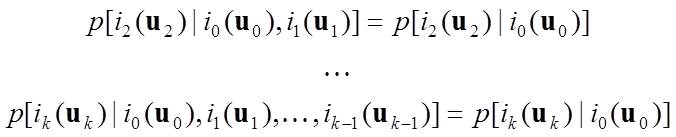
based on Bayes’ rule (Bayes 1763) and the relationship between joint probability and conditional probability. Here A is a constant, and u₁ is the last visited location or the location that the spatial Markov chain goes through to the current location u₀. Equation (2) is regarded as the full general solution of the local conditional probability distribution of MCRFs. From the Bayesian perspective, the left-hand side of the equation is the posterior probability distribution, the last term in the right-hand side is the prior probability distribution, and the remaining part of the right hand side excluding the constant is the likelihood component. The likelihood component comprises multiple likelihood functions, each for one nearest datum except for the last visited location, as shown below:

.

These likelihood functions represent a process of sequential Bayesian updating based on different nearest data as evidence within the neighborhood. Each nearest datum represents new evidence that may be used to update the previous information about the local conditional probability distribution at location u₀ to make it closer to the truth. The updating process starts from nearest neighbor at u₂ and ends at nearest neighbor at u_m within the neighborhood around the uninformed location u₀. 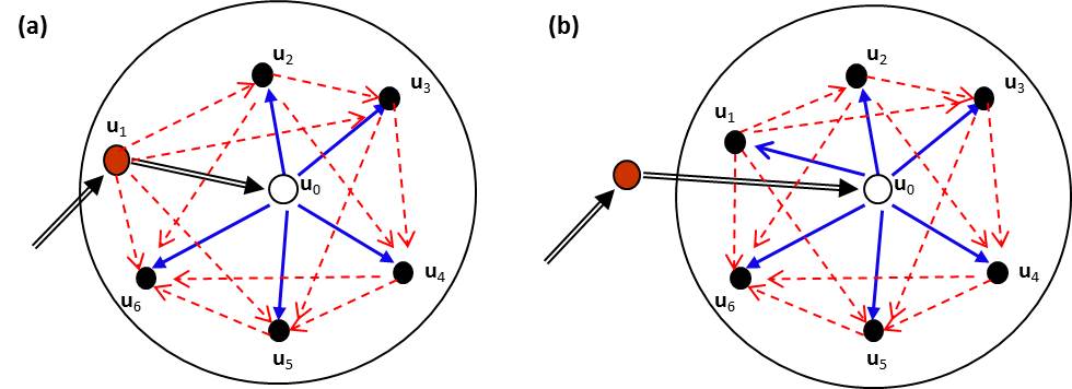Nearest neighbors used in earlier updatings in the updating sequence become the conditioning data of later updatings, and all updatings are conditioned on the variable at u₀ being estimated, as illustrated in Figure 1(a), with a neighborhood of six nearest neighbors. Such a sequential Bayesian updating on nearest spatial data within a neighborhood is one of the major characteristics of MCRFs (Li et al. 2013, 2015).

In Eq. (2), it is assumed that one of the nearest neighbors can serve as the last visited location of the spatial Markov chain. If the last visited location is far away from the current location being estimated (i.e., the last visited location is outside the neighborhood), its impact may be ignored due to the long distance and the screening effect of nearest data. In such a case, if we still consider m nearest neighbors, the local conditional probability distribution can be factorized as

(3)    

where A is a constant, and u₁ is simply a nearest neighbor (Li et al. 2015). Compared to Eq. (2), Eq. (3) has the similar sequential Bayesian updating process, but its prior probability distribution becomes a marginal probability distribution and there is one more likelihood function, in the form of

.

Eq. (3) is illustrated in Fig. 1(b), with a neighborhood of six nearest neighbors. Given the same number of nearest neighbors, Eq. (3) is equivalent to Eq. (2). Because we can assume that the spatial Markov chain always goes through a nearest neighbor to reach the current location being estimated, Eq. (2) is sufficient to be the full general solution of MCRFs.

Figure 1. Data interactions in local neighborhoods of Markov chain random fields (MCRFs). The data interactions within a neighborhood essentially form a full "Bayesian network" of local spatial data points (plus the unobserved location being estimated), but no causality can be used to build such a "spatial" Bayesian network: (a) A standard MCRF neighborhood with six nearest neighbors and data interactions (assuming u₁ is the last visited location of the spatial Markov chain). (b) The same neighborhood but the last visited location is assumed to be far away (outside the neighborhood). The data interactions also show the local sequential Bayesian updating process. Data interactions across the uninformed location u₀ being estimated are ignored based on Markov property and for clarity of illustration.

In Eqs. (2) and (3), the likelihood functions include a series of three-point to m+1-point likelihood functions that involve the unobserved location u₀. Consequently, the full general solution of MCRFs is essentially a spatial model of multiple-point statistics (actually mulitple-point likelihoods) at the neighborhood level. But the multiple-point spatial model we suggested here by using Bayesian factorization of nearest spatial point data within a neighborhood is theoretically different from the existing multiple-point geostatistics. Our multiple-point model is a neighborhood-level sequential Bayesian updating model with multiple-point likelihoods.

The multiple-point likelihoods in above equations are also functions of separate distances because these data points may not be immediately adjacent in a sparse or inexhaustive data space. Without simplification, the likelihood functions involving multiple data points are difficult to estimate from sparse sample data.

Figures 1(a) and 1(b) are visualizations of Eqs. (2) and (3), respectively, and as Bayesian models they are probabilistic directed acyclic graphs. Therefore, MCRF theory essentially conforms to Bayesian networks (Pearl 1986), which are formally probabilistic directed acyclic graphs. However, considering MCRFs as traditional Bayesian networks is not reasonable. Bayesian networks (Pearl 2000) are typically characterized by cause-consequence relationships, where causes are represented by parent nodes and consequences by children nodes. Based on the parent-child relationships in a graphic representation, a probabilistic mathematical model can be derived. Therefore, Bayesian networks can help to build probabilistic models. However, there are no such cause-consequence (or parent-child) relationships among spatial data points. Thus, to correctly construct a Bayesian network for a set of spatial data points is difficult. In fact, without first having Eqs. (2) and (3), we even would not have been able to draw the graphic networks in Figs. 1(a) and 1(b) for illustrating the two equations in the first place. This is probably why Bayesian networks have been rarely used for building spatial correlation models of spatial sample data. In addition, Bayesian networks do not provide a way to deal with distant data interactions. Fortunately, the idea of “using a single spatial Markov chain to deal with a whole random field with sample data” plus the idea of "sequentical Bayesian updating on nearest data within a neighborhood" overcame the challenge of causality (Li 2007a).

It is worth mentioning that the Bayesian updating (or inference) philosophy was not unknown in geostatistical modeling; however, earlier studies (Omre 1987; Woodbury 1989; Christakos 1990; Banerjee et al. 2004) mainly used it for parameter estimation or for incorporation of soft information, rather than for factorizing a univariate local conditional probability distribution to each of nearest data points, as done in MCRFs.

Simplified MCRF models with conditional independence assumption

Conditional independence is a practical assumption widely used in Bayesian analysis of non-spatial data (Dawid 1979; Pearl 2000). Bayesian networks for non-spatial data (events) widely used the conditional independence assumption. For spatial data, conditional independence of nearest neighbors within a neighborhood rarely holds. Even so, practical use of the conditional independence assumption to spatial data is still feasible for simplifying models or computation, if conditioning data and neighborhoods are not strongly asymmetric, as suggested in Li (2007) and used in Li and Zhang (2007). In fact, this assumption theoretically holds in Pickard random fields for immediately adjacent cells in cardinal directions given the value of the central cell on a regular lattice (Pickard 1980; Rosholm 1997; Li 2007), and it is also applicable to sparse sample data in cardinal directions (Li 2007a). The generalized conditional independence assumption used here for spatial data assumes that given the value of the random variable at the location u₀ its nearest neighbors in different directions are conditionally independent (Li 2007a). Thus, we have

(4)    

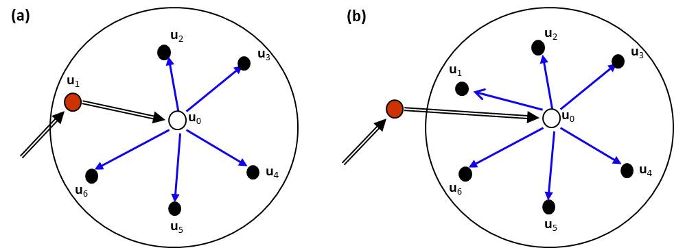
With such a conditional independence assumption applied, all of the likelihood terms in Eq. (2) become two-point conditional probabilities, and Eq. (2) can be simplified (Li 2007a) to

(5)    

Figure 2(a) illustrates this simplified MCRF solution with a neighborhood of six nearest neighbors. Similarly, Eq. (3) can be simplified to

(6)    

which is illustrated by Fig. 2(b).

Figure 2. Data interactions in local neighborhoods of simplified MCRF models based on the conditional independence assumption of nearest neighbors: (a) A neighborhood with six nearest neighbors and data interactions (assuming u₁ is the last visited location of the spatial Markov chain). (b) The same neighborhood but the last visited location is assumed to be far away (outside the neighborhood).

It is obvious that Figures 2(a) and 2(b) are still probabilistic directed acyclic graphs, that is, Bayesian networks on spatial data. Due to the complex spatial correlations among spatial data, Eqs. (5) and (6) do not truly hold for real spatial data. The degrees of their departures from the real conditional independence of nearest neighbors largely depend on the numbers and spatial configurations of nearest neighbors.

Simplified MCRF models with the transiogram notation

The two-point conditional probabilities in the right hand sides of Eqs. (5) and (6) are essentially spatial transition probabilities over their respective separate distances (i.e., spatial lags). For example, p[i_m(u_m)|i₀(u₀)] can be written as p_i0im(h_0m) with h_0m = u_m - u₀. For a continuous variable h_0m, p_i0im(h_0m) is a transition probability function. Assuming second-order stationarity on spatial data (Cressie 1993), such a spatial transition probability function does not depend on specific spatial locations and may be used as a measure to describe the spatial correlation of categorical spatial data. For the convenience of description and following the variogram concept (Matheron 1963; Goovaerts 1997), the transition probability function over a spatial lag variable, generally written as p_ij(h), was named as the transiogram (Li 2007b). Thus, a transiogram is theoretically expressed as

(7)    

where i and j denote the specific states (i.e., classes) of random variables Z(u) and Z(u+h) at locations u and u + h, respectively. Similar to the variogram, the transiogram p_ij(h) is graphically a curve with increasing h from zero. The transiogram expression in Eq. (7) is identical to the spatial transition probability function in Luo (1996, p. 284). It is well known that similar spatial transition probability functions were applied to indicator kriging formulas by Carle and Fogg (1996). However, the transiogram in our study is not simply a transition probability-lag function expression as p_ij(h). 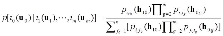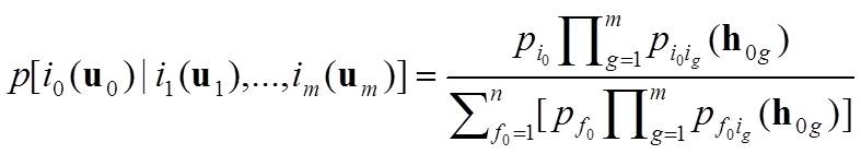It is a component to constitute the simplified MCRF models, and a methodology for providing transition probability values to implement the simplified MCRF models.

With the spatial second-order stationarity assumption and the transiogram notation, as well as the law of total probability, Eq. (5) can be rewritten (Li 2007a) as

(8)    

where p_i0ig(h_0g) represents a transition probability from class i₀ to class i_g with a separate distance h_0g, which can be fetched from a transiogram model; i₁(u₁) represents the nearest known neighbor from or across which the spatial Markov chain moves to the current uninformed location u₀; m represents the number of nearest known neighbors including the last visited location; i and f represent states (or classes) in the state space S = (1, …, n). Equation (8) represents the simplified general solution of MCRFs with the transiogram notation and the second-order stationarity assumption (Li 2007a). It is still in the Bayesian inference formula, with p_i1i0(h₁₀) being the prior probability, the denominator being the normalizing constant and the remaining part of the right hand side being the likelihood component.

Similarly, Eq. (6) also can be rewritten using the transiogram notation with the spatial second-order stationarity assumption as

(9)    

where p_i0 is the marginal probability of class i₀. Here p_i0 is also assumed to be spatially stationary, and it is actually the class proportion of class i₀. Equation (9) also can be directly derived from Eq. (8) by using the detailed balance principle, which assumes a reversible stationary Markov chain (Feller 1957). Thus, Eq. (9) is a special case or variant of Eq. (8). Equation (9) is still in the Bayesian inference formula, but its prior becomes the marginal probability p_i0.

Both Eq. (8) and Eq. (9) do not consider the effects of data clusters and data deviation from conditional independence. Apparently, clustered nearest neighbors deviate more from conditional independence than do non-clustered nearest neighbors, and nearest neighbors above the number of cardinal directions deviate more from conditional independence than do nearest neighbors at or below the number of cardinal directions. These situations may affect the estimation of local conditional probability distributions. Consequently, dealing with these issues in the simplified MCRF models under the conditional independence assumption may be necessary in algorithm design about neighborhood structure (e.g., using quadrant neighborhood search as done in Li and Zhang (2007)) or by adding adjusting parameters.

The full and simplified general solutions of MCRFs cover any-dimensional spaces from 1D to 3D and even 4D (spatiotemporal). In one dimension, a MCRF can be a traditional 1D Markov chain (moves one step once), or a jumping Markov chain (moves multiple steps once) or a Markov chain conditioned on nearest data at both sides. 1D to 3D specific simplified MCRF models (considering nearest data only in cardinal directions) were also provided in Li (2007a).

Varied forms of MCRF models, especially more complex and integrative models, may be developed based on the basic full and simplified solutions of MCRFs for various application purposes. For example, the full solutions of MCRFs can be partially simplified, the coMCRF model can be constructed for incorporating ancillary variables (Li et al. 2015), and other information or constraints also can be incorporated for a specific application purpose such as land cover post-classification from remote sensing imagery (Zhang et al. 2017). In addition, transition probabilities in simplified MCRF models might be replaced by other two-point spatial measures (e.g., indicator covariance) based on their quantitative relationships (Luo and Thomsen, 1994; Carle and Fogg, 1996). However, it is apparent that the transiogram is more intuitive to explain and more flexible in joint model-fitting than are other two-point spatial measures.

Remarks

The MCRF approach, especially the MCRF theory, is based on the single-Markov-chain random-field idea with integration of related knowledge in conventional Markov chain theory, Bayes' theorem, and spatial/geo-statistics, as well as some other new ideas. Mathematically, it may look "simple" in its equations and derivation; but as a spatial statistical method for conditional simulation of categorical fields conditioned on spatial sample data, it is novel and not so "simple". We are happy to see that the ideas for building the MCRF approach have caught attentions in the fields of spatial/geo-statistics and mathematical geosciences, and inspired many studies in recent years.

We thank many experts, reviewers and editors in applied statistics (e.g., mathematical geology), soil science, GIS, and remote sensing for their helps and supports in the publication process of papers of the MCRF approach. We especially want to express our gratitude to Prof. D.M. Titterington, Prof. W.E. Sharp and Prof. R.J. Martin for their supports to the publication of the MCRF idea during 2005 to 2006.

References:

Banerjee S, Carlin BP, Gelfand AE (2004) Hierarchical modeling and analysis for spatial data. CRC Press.

Bayes T (1763) An essay towards solving a problem in the doctrine of chances. Phil Trans Royal Soc London 53: 330-418.

Carle SF, Fogg GE (1996) Transition probability-based indicator geostatistics. Math Geol 28(4): 453-476.

Christakos G (1990) A Bayesian/maximum-entropy view to the spatial estimation problem. Math Geol 22(7): 763-777.

Cressie NAC (1993) Statistics for Spatial Data. Wiley, New York.

Dawid AP (1979) Conditional independence in statistical theory. J Roy Stat Soc Ser B 41(1): 1-31.

Goovaerts P (1997) Geostatistics for natural resources evaluation. Oxford university press, New York.

Feller W (1957) An Introduction to Probability Theory and Its Applications. Vol. 1, 2nd ed. John Wiley, New York.

Gelman A, Carlin J, Stern H, Rubin DB (1995) Bayesian data analysis. Chapman and Hall, London.

Jaffray JY (1992) Bayesian updating and belief functions. IEEE Trans Syst Man Cyber 22(5): 1144-1152.

Li W (2007a) Markov chain random fields for estimation of categorical variables. Math Geol 39: 321–335.

Li W (2007b) Transiograms for characterizing spatial variability of soil classes. Soil Sci Soc Am J 71: 881-893.

Li W, Zhang C (2007) A random-path Markov chain algorithm for simulating categorical soil variables from random point samples. Soil Sci Soc Am J 71(3): 656-668.

Li W, Zhang C (2008) A single-chain-based multidimensional Markov chain model for subsurface characterization. Environ Ecol Stat 15(2): 157-174.

Li W, Zhang C, Dey DK, Willig MR (2013) Updating categorical soil maps using limited survey data by Bayesian Markov chain cosimulation. Sci World J. Article ID 587284. doi:10.1155/2013/587284.

Li W, Zhang C, Willig MR, Dey DK, Wang G, You L (2015) Bayesian Markov chain random field cosimulation for improving land cover classification accuracy. Math Geosci 47(2): 123-148.

Luo J (1996) Transition probability approach to statistical analysis of spatial qualitative variables in geology. In: Forster A, Merriam DF (eds.) Geologic modeling and mapping (Proceedings of the 25th Anniversary Meeting of the International Association for Mathematical Geology, October 10-14, 1993, Prague, Czech Republic). Plenum Press, New York. p. 281–299.

Matheron, G (1963) Principles of geostatistics. Economic Geol 58: 1246-1266.

Omre H (1987) Bayesian kriging - Merging observations and qualified guesses in kriging. Math Geol 19(1): 25–39.

Pearl J (1986) Fusion, propagation, and structuring in belief networks. Artificial intelligence, 29(3), 241-288.

Pearl J (2000) Causality: Models, Reasoning, and Inference. Cambridge University Press.

Pickard DK (1980) Unilateral Markov fields. Advances in Applied Probability 12(3): 655–671.

Rosholm A (1997) Statistical methods for segmentation and classification of images. Ph.D. dissertation, Technical University of Denmark, Lyngby.

Woodbury AD (1989) Bayesian updating revisited. Math Geol 21(3): 285-308

Go Back