Go Back
The single-Markov-chain random-field idea
The MCRF approach (i.e. Markov chain geostatistics) was essentially built on the "single-Markov-chain random-field idea". This idea is very different from conventional Markov random fields (MRFs) defined on regular or irregular lattices. It is a locally-conditioned Markov chain. It was found later that such a model conforms to a special spatial Bayesian network over a neighborhood. This means that MCRF models (both the full and simplified forms) can be regarded as neighborhood-based special spatial Bayesian networks on (sparse) spatial data.
In fact, our first manuscript for the MCRF approach was the initial manuscript of Li and Zhang (2008), which proposed a single-chain-based multidimensional Markov chain model for correcting the theoretical problem of the coupled Markov chain (CMC) model for subsurface characterization. Unfortunately, the manuscript did not get published in time due to some reasons. This manuscript was first submitted to a top statisticial journal (Journal of the Royal Statistical Society: Series B) in September 2004 by mail, with the hope to get some suggestions from reviewers in spatial statistics. It was not sent out for review by the journal (see the response letter from the editor). Then it was submitted to a water resource journal (Water Resources Research), but was severely misunderstood by reviewers in hydrogeology. Later I submitted it to another prestigious statistical journal (Biometrika). The editor-in-chief of the journal at that time was a well-known spatial statistician. He read the manuscript, thought our work was a good idea, and encouraged me to submit it to an applied statistical journal (see the response letter from the editor). His appreciation to the model encouraged me very much, making me later not giving up the effort to publish the ideas of the MCRF approach and further develop them into practical methods, even though we met larger difficulties later. I submitted it to Environmental and Ecological Statistics, which finally published it after a long review process by three reviewers in spatial statistics, who all confirmed the value of the model. Of course, repetitive revisions (including manuscript title and model name) were made during the whole submission and revision process for publishing the article. This single-chain-based multidimensional Markov chain model (previously called "spatial Markov chain models") was based on the single-Markov-chain idea and the spatial conditional indepednece property of nearest neighbors in cardinal directions in a Pickard random field. It seemed simple, but it was novel and unique for geostatistics. More importantly, it seemed that it solved well the major problem (i.e., small class underestimation) of the coupled Markov chain (CMC) model suggested by Elfeki and Dekking (2001). The MCRF model presented in Li (2007a) was a generalization of the single-chain-based multi-D Markov chain model, based on the generalized single-Markov-chain idea. The initial manuscript of Li (2007a) was submitted to another top statistical journal in October 2004, but not sent out for review by the journal editors, partially because the application case study was too simple (we had no conditions and time to develop a more practical simulation algorithm and a software system at that time, so we only did a simple simulation of a 2-D soil texture layer vertical section). In addition, some non-spatial statisticians thought the MCRF model (or single-chain-based multi-D Markov chain model) was very simple (not sufficiently developed in statistics) and statistically might not have high value, especially we were not statisticians. But our purpose was to solve existing scientific problems in Markov chain spatial modeling; pure statistical issues were not our concern. Our limited knowledge in statistics made us only able to describe the model with simple equations and mainly with descriptions in words based on our knowledge. It seems there are different understandings to geo/spatial-statistics between nonspatial statisticians and geo/spatial-statisticians, which is quite understandable. People who did not work on spatial data (especially sparse sample data) may not understand the special nature of spatial data and the complexity and difficulty in dealing with spatial data, and might feel that geo/spatial-statistical models were just simple adaptions of nonspatial statistical models (e.g., purely from the angle of statistical equations, some people might think kriging was a simple adaption of multiple linear regression). Later the manuscript was submitted to Mathematical Geology in December 2004, and finally got published after a long review process. The single-Markov-chain random-field idea was not only a new idea but also extended the conventional Markov chain theory into a theoretically-strict geostatistical approach for conditional simulation of categorical fields (consequently solved the deficiencies of the CMC model). From this angle, it should represent an important progress in geo/spatial-statistics. Its application value depends on how we use it and expand it for specific application purposes. To be honest, we never had the desire to create a new geostatistical model or approach until I realized that we had already made it in ideas (already wrote it in manuscripts and partially implemented it), because both my education background and my previous research interests were not geo/spatial-statistics (I just used 1-D Markov chains and kriging to study soil textural layer vertical sequences, clay layer thickness and clay layer emerging depth in my PhD dissertation in early 1990s). It is because we accidentally encountered some scientific issues in application study using the 2-D CMC model in 1999 that we began to study geo/spatial-statistics and explore how to solve the scientific issues we met in multi-D Markov chain modeling, and eventually we solved them. It is the huge amount of fundamental research work in a long-time process with scientific integrity and conscience that made the MCRF approach! The MCRF theory might not be a perfect theory at the beginning, but it proved to be very justifiable and self-explaining. More importantly, it is a typical problem-solving study and the approach has been proven to be practical in application studies.
Single-Markov-chain random field
The reason that we have such an idea came from our earlier studies in using and modifying (extending) a 2D coupled Markov chain model, which coulpled two 1D Markov chains together. Our studies showed that the model underestimated small classes. We found that it is an intrinsic problem of the model and we believed that the small class underestimation problem should be caused by the exclusion of conflict transitions (i.e., unwanted transitions) when coupling two Markov chains (Li 2007a, Li and Zhang 2008). Therefore, multi-D nonlinear Markov chain models built on the idea of coupling two or more 1D Markov chains all have the small class underestimation problem, and the problem becomes severer with increasing number of conflict transitions. We tested all of those model choices, such as coupled Markov chains, tripled Markov chains, and quadrupled Markov chains. This study gradually led me to the question - How about to use a single Markov chain to do the multi-D simulation? I was not the only person who thought of that point. A reviewer who reviewed our manuscript submitted to a water resources journal in 2003 also mentioned this point in his/her comments, as he/she stated that "Somebody ever said we probably should use a single Markov chain to do multi-D simulation, but nobody knows how to do it". I finally had time to concentrate on thinking about this idea, after my research in multi-D Markov chain modeling lost support (and soon our NSF project application also failed in June 2004) in UW-Madison and after my wife and I moved to live at Whitewater, Wisconsin, in the summer of 2004. However, when I finally developed the random-path simulation algorithm, it was already Spring 2006.
By assuming there is only a single Markov chain in a space, we can avoid the conflict transitions caused by using multiple 1-D Markov chains. Then the small class underestimation problem may be overcome. Further, by assuming the single Markov chain can jump within a space from one location to another like a Brownian motion (thus, moving step by step following a fixed path becomes a special case), the Markov chain simulation process can be generalized to a situation of spatial sequential simulation with a random path. The remaining difficulty, also the key, was how to incorporate the interactions of the Markov chain with nearest data in different directions within a neighborhood around an unobserved location into the spatial Markov chain. I found that by using the Bayes' theorem and the relationship of conditional probability and joint probability, I could factorize the neighborhood data to an extent that each of these nearest data become a piece of new information for updating the initial (i.e., prior) probability distribution of the categorical random variable at the unobserved location, and the cardinal-neighbor conditional independence property of Pickard random fields could be further extended and used to simplify the model into a form without multiple-point terms. The modified Markov chain model obtained by such a way has no conflict transitions.
Assume that a categorical random field Z{Z(x): x∈D} has N unobserved locations and M observed locations, and the random variable Z(x0) at an unobserved location x0 has m nearest data neighbors in different directions. Here we use i (i=1,...,n) to denote the state (i.e., class) of a categorical random variable. Then the local conditional probbaility distribution of the random field Z{Z(x): x∈D} at the location x0 can be generally denoted as p[i(x0)|i(x1),...,i(xm)], and the joint probability distribution of the random field Z{Z(x): x∈D}, conditioned on the M observed data, can be given as
(1) ![]()
for a set of specific states for all unsampled locations. However, to conduct conditional simulations, what we need is how to solve the generalized local conditional probability distribution function, p[i(x0)|i(x1),...,i(xm)], rather than how to write the joint probability distribution.
The above single-Markov-chain random-field idea was illustrated in figure 1 in Li (2007a). Let's show it here again as Figure 1a, and provide some more explanations (Figure 1b). A single Markov chain, as denoted by the solid arrow, jumps in an any-D space. At each unobserved location it arrives, it interacts with nearest data neighbors in different directions to decide its local conditional probability distribution and consequently its state. The nearest data neighbors around an unobserved location constitute a local neighborhood. There are three neighborhoods in Figure 1a, as highlighted in Figure 1b. In the first neighborhood (NH1), the last visited location is within the nearest neighbors. For the second neighborhood (NH2), the last visited location is not within nearest neighbors because it is far away, outside the neighborhood. For the third neighborhood (NH3), the last visited location is also not within the neighborhood, but the Markov chain moves through a nearest neighbor x1. Thus, the nearest neighbor crossed by the Markov chain replaces the last visited location. In general, one may always consider a last visited location (assume one nearest neighbor to be it) or not consider it (assume the last visited location to be far away). Labels x1 to x7 were used to denote the nearest neighbors (both locations and states) in Li (2007a). In above and below equations, we use i(x) to denote the state of a categorical random variable at location x. In addition, in Figure 1, as it was shown originally in Li (2007a), we did not draw the lines for the interactions between nearest data neighbors [kriging neighborhoods were usually similarly illustrated, though they consider interactions between nearest data (i.e., data configuration) in estimating the data weights. The difference is that kriging neighborhoods do not emphasize the Markov property (there is Markov-type kriging which uses Markov-type neighborhood)], but interactions between nearest data neighbors do exist before we make simplification using the spatial conditional independence assumption of nearest neighbors. To avoid misunderstandings, these data interaction lines were clearly drawn in our later articles - Li et al. (2013, figure 1) and Li et al. (2015, figure 2).
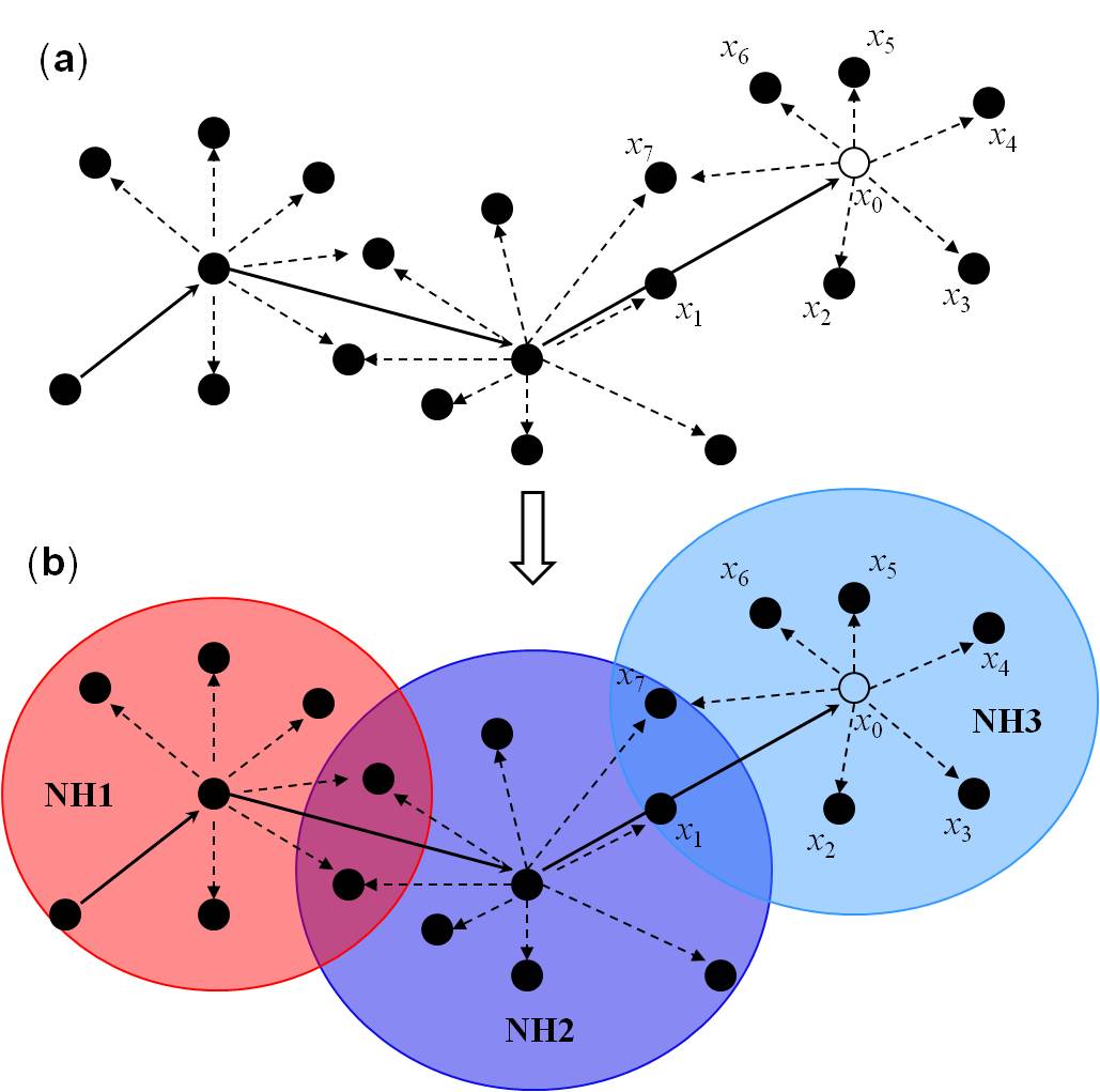
Figure 1. Illustration of a Markov chain random field. (a) A Markov chain jumps in a multi-D space from one unobserved location to another, and interacts with nearest data neighbors (from Li 2007a, p.325). (b) The three neighborhoods (i.e., NH1, NH2 and NH3) with different situations of the last visited location are highlighted. The empty cell denotes the current state-unknown location, and surrounding black cells represent its nearest data neighbors in different directions in a search area. Arrows represent directional interactions (i.e., transition probability tail-head directions). The solid arrows also represent the moving directions of the Markov chain. After the Markov chain moves to next location, the current location becomes informed.
Local conditional probability distribution
Solving the local conditional probability distribution function p[i(x0)|i(x1),...,i(xm)] of MCRFs is the core for implementing the single-Markov-chain Markov field idea. But how to solve it? Because using multiple 1-D Markov chains one per direction is not a suitable choice, I chose using Bayes's theorem and the relationship between conditional probability and joint probability to factorize the local conditional probability function to each nearest data point. The factorized equation involves some complex multi-point conditional probabitlies (actually likelihoods), which cannot be easily estimated from sample data. So spatial conditional independence assumption was used to simplify the model. The spatial conditional independence assumption of nearest data within a neighborhood was also presented in Li (2007a).
The factorization of the local conditional probability distribution function generates
(2) ![]()
At the same time, I also found that the local conditional probbaility distribution function could be factorized as
(3) ![]()
Above EQ (3) can perfectly explain the single-Markov-chain idea (with the last visited location being within the neighborhood), while EQ (2) can be regarded as a special case (with the last visited location not being within the neighborhood). So EQ (3) was chosen as the full general solution of MCRFs, because we can always assume one of the nearest neighbors to be the last visited location. However, when drawing the figure for illustrating the MCRF idea in Li (2007a), all three neighborhood cases were drawn (see Figure 1b). In above Figure 1b, both NH1 and NH3 illustrate EQ (3), but NH2 illustrates EQ(2). To avoid "misunderstandings", later we had to include both EQ (3) and EQ (2) in the MCRF theory and the nearest data interaction lines within a neighborhood also had to be clearly drawn.
The above factorization of nearest point data within a neighborhood seems very simple. However, it contains the philosophical thought of Bayesian updating based on new evidence provided by each data point within a neighborhood. Such a use of Bayesian updating to the nearest data within a neighborhood (i.e., spatial sequential Bayesian updating on nearest data) should be a new idea in geostatistics (we have not seen an earlier similar use).
Above EQ (3) and EQ (2) are essentially multiple-point spatial models. But the multiple-point spatial model we suggested here is different from the existing multiple-point geostatistics in both theory and formula; the latter was initially derived from the extended indicator kriging framework (Guardiano and Srivastava 1993). Our multiple-point spatial model is a neighborhood-level nonlinear sequential Bayesian updating model using multiple-point likelihoods. To implement above MCRF models using only sample data, we had to simplify these multiple-point likelihoods to two-point statistics so that parameters can be directly estimated from sample data. The conditional independence property of adjacent cells in cardinal directions in Pickard random fields was extended to the sparse sample data situation for this purpose. Although the ordinary conditional independence assumption was used in Bayesian statistical analysis for non-spatial data ( i.e., various events, no matter whether they are categorical or not, and no matter whether they have the same nature), it was rarely used on spatial data in geo/spatial-statistical models, especially on sparse data points. With the second-order stationarity assumption, the transiogram notation (i.e., transition probability-lag function) was further used to expresss the MCRF models simplified by the spatial conditional independence assumption of nearest data (see the page for MCRF theory) and transiogram models were used to provide transition probability parameters to simplified MCRF models.
Remark: Although the MCRF idea emphasized the Markov property (see the Markov-type neighborhood in above Figure 1), the MCRF idea and the conventional MRF idea are different. The conventional MRF model is equivalent to a Gibbs distribution, which comprises a set of cliques (from single-node cliques to multi-node cliques), and it is normally used as a lattice model without directly dealing with sample data and distant interactions. Even drawn as a graph, MRFs are undirected graphs. However, the purpose of the MCRF approach is mainly for directly dealing with sample data and distant interactions. One may regard the MCRF approach as an extension of conventional MRFs toward sparse data space where distant interactions need to be considered, if they want; but this does not mean that they can be derived from each other, because the generalized form of MCRF models was derived by decomposing the joint probability distribution of a spatial random variable and its neighborhood through sequential Bayesian updating and thus it is essentially a neighborhood-based special spatial Bayesian network. Therefore, a MCRF model is a locally-conditioned Markov chain and also a special spatial Bayesian network on spatial data. The derivation process of the MCRF model only needs some knowledge in conventional 1-D Markov chain theory, Bayes' theorem (Bayesian updating), conventional geostatistics (kriging and variogram), and pioneer studies in Markov chain spatial modeling.
References
Guardiano, F., Srivastava, R.M. 1993. Multivariate Geostatistics: Beyond Bivariate Moments, in Soares, A., ed., Geostatistics-Troia, Kluwer, Dordrecht, vol. 1, p. 133-144.
Li W (2007a) Markov chain random fields for estimation of categorical variables. Math Geol 39: 321–335.
Li, W., Zhang, C. 2008. A single-chain-based multidimensional Markov chain model for subsurface characterization. Environmental and Ecological Statistics, 15(2): 157-174.
Li W, Zhang C, Dey DK, Willig MR (2013) Updating categorical soil maps using limited survey data by Bayesian Markov chain cosimulation. Sci World J. Article ID 587284. doi:10.1155/2013/587284.
Li W, Zhang C, Willig MR, Dey DK, Wang G, You L (2015) Bayesian Markov chain random field cosimulation for improving land cover classification accuracy. Math Geosci 47(2): 123-148.