Go Back
Transiograms
The transiogram method was mainly developed for implementing MCRF models as part of the MCRF approach. The “transiogram” term was created to specifically express a transition probability-lag function or curve for the convenience of use (Li 2007), in order to avoid terminological confusions (for example, a "transition probability" normally means a single value, the term of "Markov diagram" or "transition probability diagram" has been traditionally used for the graphs of transitions between different states in non-spatial or 1D Markov chains). But the transiogram is not just a short-name. As a spatial correlation measure for spatiotemporal categorical variables connected with Markov chain theory, it is also a methodology. As a transition probability-lag function, the transiogram is the basic component to constitute simplified MCRF models. The transiogram concepts followed the style of variogram concepts. Its essence lies with the interpretation of physical meanings of transiogram features (e.g., range, shape) and the joint modeling of experimental transiograms for providing proper parameters to geospatial statistical simulation. Such a transiogram concept system is necessary for the MCRF approach. While this concept provided the convenience and clarity in description and understanding, it also expressed our respect to pioneers in classical geostatistics.
There are some earlier studies involving transition probability-lag curves or functions, which are related to transiograms. These pioneer studies should be respected, even if some of them were preliminary, might not be much useful to the MCRF approach, or did not get our attentions at the beginning. The variogram spatial measure in classical geostatistics provides a reference to the development of the transiogram as a spatial measure. In the following sections, we provide a simple introduction of the main contents of the transiogram in our study. We specifically introduce related earlier studies in another page. Readers may go to Li (2007), Li and Zhang (2010) and Li et al. (2012) for more details about transiograms.
The transiogram may be used as an independent spatial measure for correlation analysis of categorical variables. It may also be used in other approaches if one would like.
1. Definition and concepts
With the second-order stationarity assumption, the two-point conditional probabilities in the simplified MCRF models based on the conditional independence assumption are essentially spatial transition probabilities over their respective two-point separate distances, that is, transition probability functions of the spatial lag h, because the nearest data points are normally located with a distance from the unobserved location being estimated. Such a spatial transition probability function does not depend on specific spatial locations and may be used as a measure to describe the spatial correlation of a pair of classes. For clarity and convenience of description, it was named as the transiogram, simplified from the transition probability diagram (Li 2007). Thus, a transiogram is theoretically defined as a two-point transition probability function over the separation distance (i.e., spatial lag), generally written as pij(h) with
(1) ![]()
where i and j denote the specific states (i.e., classes) of random variables Z(u) and Z(u+h) at locations u and u + h, respectively. Similar to the variogram, the transiogram pij(h) is graphically a curve with increasing h from zero. The transiogram expression in Eq. (1) is identical to the spatial transition probability-lag function in Luo (1996, p. 284).
Please note that here the transiogram is directly defined as a transition probability-lag function theoretically, rather than a two-point joint probability-lag function or a two-point conditional probability-lag function derived from a two-point joint probability-lag function. Because a two-point joint probability is symmetric and a two-point conditional probability derived from a two-point joint probability cannot be unidirectional (e.g., from left to right or from top to bottom), they lose some special properties of transition probabilities and may not be explained using stationary 1D Markov chain theory (or transition probability matrix). To avoid those issues, we defined the transiogram as a transition probability-lag function theoretically and as a transition probability-lag diagram visually, so that it is purely a transition probability-based spatial measure within the framework of Markov chain theory and mainly serves Markov chain spatial models. In addition, the transiogram definitation here is irrelevant with indicator variables. If indicator variables are invovled, they are treated as binary categorical variables.
The concepts about the transiogram follows the style of the concepts about the variogram so that it is easy to understand and convenient to use (e.g., for description in Markov chain spatal modeling). So we have: auto/cross transiograms, experimental (or empirical or sample) transiograms, theoretical transiograms or transiogram models, sills and ranges. But there are differences: (a) Because cross transiograms are asymmetric and can be unidirectional, they have tail and head classes. (b) Transiograms can be directly calculated from a single-step transition probability matrix if it is available, and such transiograms are called idealized transiograms because they are very smooth curves produced by the computation equation based on the stationary Markov assumption on spatial data (Li 2007). Idealized transiogram has no counterpart in classical geostatistics. Although idealized transiograms miss the complex feastures of experimental transiograms, they are useful for understanding the experimental transiograms if they are available. In addition, they may be used directly (or indirectly through a linear interpolation) as simple transiogram models if avaiable, when more practical transiogram models are not available. Similar to experimental variograms, experimental transiograms are directly estimated from sample data.
Note that in classical geostatistics, the term cross variogram is used in cokriging for representing the cross correlation between a primary variable and an ancillary variable. In indicator kriging, cross indicator variograms usually means similar things. Because full indicator kriging (i.e., indicator cokriging of multiple classes) was rarely used, cross indicator varograms between classes of the same categorical field are rarely studied in geostatistical literature. In the MCRF approach, cross transiograms represent the cross correlations between classes of the same categorical field. For incorporating ancillary variables, the cross transiograms (and cross transition probabilities) used are called “cross-field transiograms” (and cross-field transition probabilities) (Li et al. 2013, 2015). Cross-field transition probabilities have no auto transition probabilities and they may not form a square matrix.
2. Joint modeling methods
To obtain a whole set of transiogram models for performing MCRF simulation of a multi-class categorical field, we need to derive the set of transiogram models jointly (or model-fit the experimental transiograms jointly) so that transiogram models can meet the constraint – each row of transiogram models in a transiogram matrix must sum to unity at any lag value.
We proposed two methods for such a purpose (i.e., coregionalization of multiple classes) . One is a parametric method, which uses math models to fit individual experimental transiograms, but in each row of a transiogram model matrix one model must take the left portion of one minus other models, as
(2) ![]()
This method may need repetitive tuning to ensure the left model to be non-negative and well-fitted. It seems that the repetitive tuning process is annoying, but practically it is not difficult. As long as other models are rationally fitted, it is easy to get the left model well-fitted. This method is widely applicable, but may be tedious when a large number of transiorgams are involved in a simulation.
The second method is a non-parametric method, which linearly interpolates discontinuous experimental transiograms into continuous models. The equation for the linear interpolation method is given as
(3) ![]()
This method is applicable when experimental transiograms are reliably estimated, that is, when sample data are not very sparse. Otherwise, it may bring large error into simulated results. This method is very simple, but it does work and also can meet the constraints of transiogram modeling – non-negative and summing-to-unity (Li and Zhang 2010). These two transiogram joint modeling methods for coregionalization of multiple classes are practical. Both methods have been used in the model testing and application studies of MCRF methods. Pleae note that the above two joint transiogram modeling methods were proposed for the MCRF approach and were proved workable; however, they may not be suitable to the TPROGS approach suggested by Carle and Fogg (1996) due to the requirements of indicator kriging/cokriging equation systems in computation (we did not make the testing).
Carle and Fogg (1997) suggested the transition rate method for joint modeling of a whole set of transition probabilities estimated from sample data (called "experimental transiograms" in the MCRF approach). The transition rate-based coregionalization model of multiple classes was called "continuous-lag Markov chain model" (similar to continous time Markov chain model). The method is more convenient for incorporating expert knowledge, such as lithofacies mean length or thickness, and is valuable for simulating subsurface facies, where borehole sample data are usually sparse, especially in lateral directions. But when there are many sample data available, the relatively over-idealized transiogram model curve shapes from the method have difficulty to fit the complex shapes of some of experimental transiograms. Because the transiogram models generated by the method are still based on the stationary first-order Markovian assumption and their shapes are basically identical to the idealized transiograms calculated from a single-step transition probability matrix, they were regarded as idealized transiograms in Li (2007). Whether such a treatment is proper can be an issue for further study.
3. Mathematical models
Math models may be used to fit experimental transiograms to get transiogram models individually, similar to the way how they are used to fit experimental variograms in classical geostatistics. Those math models that were used to fit experimental variograms may be adapted to fit experimental transiograms. Although not specifically addressed, Carle and Fogg (1996) should be the first study that attempted to use math models to fit experimental transiograms (it mentioned that it used the sum of proportions and spherical and exponential models). In Ritzi (2000), a set of basic math models for auto transiogram (linear, spherical, exponential, Gaussian and nugget), adapted directly from variorgam models, was provided. By summarizing the work of Ritzi and some other basic math models for variogram modeling, Li (2007) provided a relatively complete set of basic math models for both auto and cross transiogram modeling, including the cosine–exponential and cosine–Gaussian composite models (i.e., hole-effect models), where the sills of transiogram models were similarly set to the coppresponding class proportions.
Although these math models may be used singly or groupedly to fit experimental transiograms, they are still not enough to capture some special feature of cross transiograms. A typical feature of cross transiograms for classes that tend to be neighbors is the peaking feature – a cross transiogram first has a peak and then gradually flattens. Because this feature occurs clearly on some idealized cross transiograms, we can judge it is a normal and rational feature for some experimental cross transiograms. This feature cannot be effectively captured by hole-effect models. To capture this feature in cross transiogram models, we suggested a set of gamma distribution based composite models (Figure 1)(Li et al. 2012). Despite the fact that these composite models have five parameters, our pratice indicated that it is not much difficult to use them in transiogram modeling. Below are the three gamma-based additive composite models (Eq. (4) for the gamma-exponential model, Eq. (5) for the gamma-Gaussian model, and Eq. (6) for the gamma-spherical model):
(4) ![]()
(5) ![]()
(6) ![]()
![]()
Figure 1. Different gamma-based additive composite models with the same parameter setting for modeling cross transiograms of neighboring classes (from Li et al. 2012).
4. Properties and features
As transition probabilities, transiograms have some common properties (Li 2007): 1) Non-negative. Probabilities cannot be negative. 2) Sum to unity. Values of a row of transiograms in a transiogram matrix (i.e., transiograms involving the same tail class) sum to 1 at any lag value. 3) Asymmetry. pij(h) is normally not equal to pji(h). However, if experimental transiograms are estimated bidirectionally or omnidirectionally, they should follow the detailed balance principle. 4) Irreversibility. If experimental transiograms are estimated unidirectionally, they are normally irreversible, that is, pij(h) is not equal to pij(-h). 5) No nugget effect. For mutually exclusive classes, transiograms theoretically should not have nugget effect.
Idealized transiograms have the following properties, which may not hold for experimental transiograms: 1) With increasing h, an idealized auto-transiogram gradually decreases to a stable value, its sill, whch is equal to the proportion of the class in a sufficiently large area. 2) With increasing h, an idealized cross-transiogram gradually approaches a stable value, its sill, which is equal to the proportion of the head class in a sufficiently large area. 3) Both auto and cross idealized transiograms have a correlation range. 4) If we draw a tangent of the idealized auto-transiogram from point (0,1) to the x axis, the lag h where the tangent crosses the x axis is equal to the mean of the polygon size of the class (see Carle and Fogg 1996). (5) Idealized auto-transiograms usually decline exponentially. (6) While most idealized cross-transiograms gradually increase to their stable values, some may first have a peak (or even some oscillations) before becoming stable. The peak is a reflection of the neighboring characteristic of the two involved classes (Li et al. 2012). We emphasize a sufficiently large area because the boundary effect (class polygons at boundaries are not complete) may impact the sills of idealized transiograms. Although experimental transiograms directly estimated from real data may have much more complex shapes (it was regarded as non-Markov effect in Li 2007) compared with the shapes of idealized transiograms, their general trends mostly follow idealized transiograms. Hence, properties and features of idealized transiograms may help understanding and modeling experimental transiograms.
These properties mentioned above are all observable from experimental and/or idealized transiograms, as demonstrated in Li (2007) and Li et al. (2012). Idealized transiograms usually have some typical shapes, as shown in Figure 2. Experimental transiograms are much more complex, but usually also follow these typical shapes approximately if a study area is sufficiently large and relatively uniform in class occurrence.
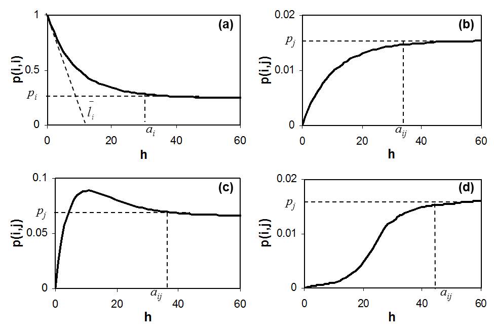
Figure 2. Illustration of typical features of transiograms (from Li 2006): (a) A typical auto-transiogram. (b) A typical cross-transiogram. (c) a typical cross transiogram for two classes that are frequent neighbors. (d) a typical cross transiogram for two classes that are rarely neighbors.
However, experimental transiograms sometimes deviate a lot from corresponding idealized transiograms (see Figure 3). When this situation occurs, idealized transiograms are improper to serve as transiogram models for categorical field smulations, even if they are available in some situations. That is why we prefer inferring transiogram models from experimental transiograms, as long as sample data are available for estimating experimental transiograms.
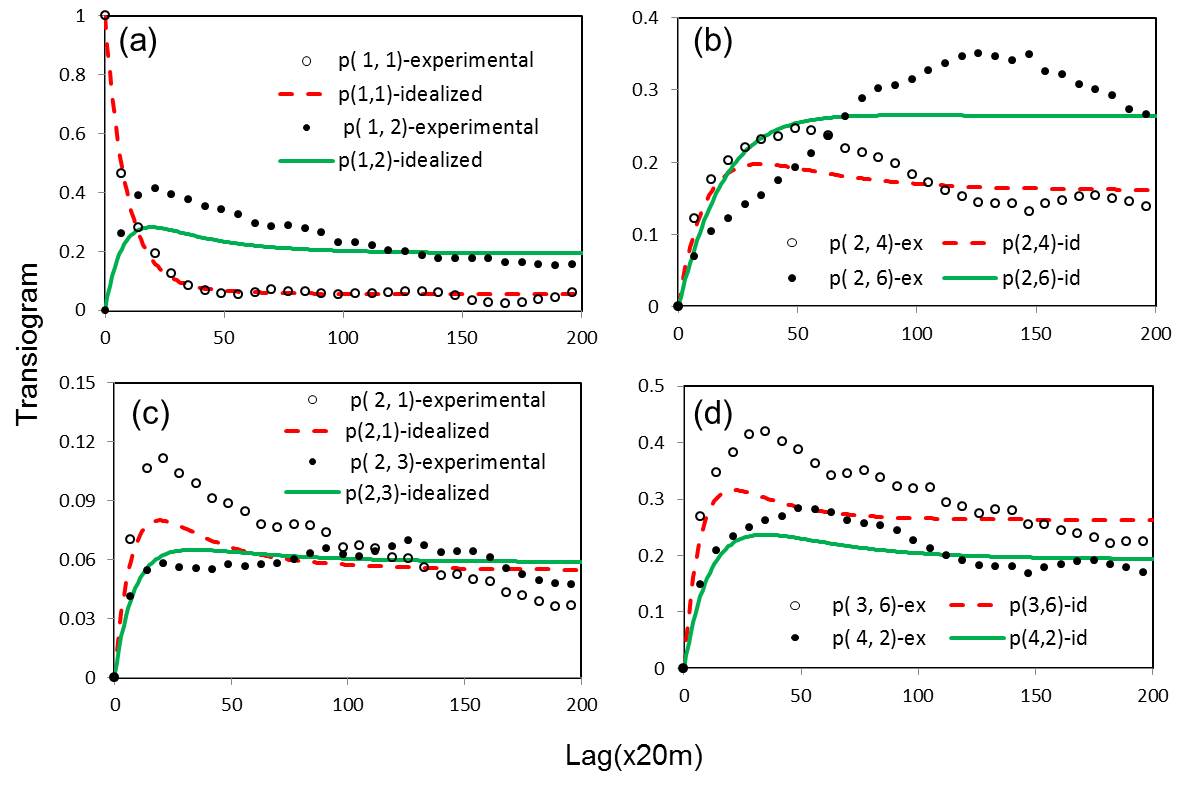
Figure 3. Experimental transiograms and corresponding idealized transiograms (from Li et al. 2012).
Remark: We thank many experts, reviewers and editors in applied statistics (mathematical geology, environmental and ecological statistics), soil science, GIS, and remote sensing for their helps and supports in the publication process of papers of the MCRF approach.
5. Misunderstandings
After the transiogram concept and methods were proposed and developed as a part of Markov chain geostatistics (mainly for implementing MCRF models), some misunderstandings emerged [e.g., some misunderstandings and self-contradiction about transiograms occurred in Cao et al. (2013), and some of them were followed by some others in statistics in China who recently attempted to publish. These misunderstandings could be possibly used by some people to create difficulties]. The following explanations clarify the major misunderstandings.
(1) One misunderstanding on the transiogram is about its definiation. During last several years (since 2012), there were some repeated attempts to redefine the transiogram with joint probability and/or indicator variables. As a transition probability-lag function/curve, the transiogram is first transition probability. Transition probability is the fundamental element in Markov chain theory, and it can be directly estimated from sample data. There is no necessity to derive a transition probability from a joint probability through the relationship between conditional probability and joint probability. Although a transition probability is a two-point conditional probability, transition probability has its special properties and meanings within Markov chain theory and it is normally used within a matrix (i.e., transition probability matrix). That is why the concept of "transition probability" emerged when Markov chain theory was proposed one hundred years ago, while "conditional probability" as a concept had existed for a long time. Redefining the transiogram through a joint probability-lag function would eliminate the legitimacy of cross transiograms to be unidirectional. In addition, transition probabilities directly describe discrete/categorical variables. There is no necessity to first turn a categorical data set (with multiple classes) into multiple sets of indicator data (i.e., 0 and 1 values) and then use indicator data to estimate transition probability and transiogram. Carle and Fogg (1996) connected transition probability with indicator variables, indicator covariance and indicator variograms; that is because the objective of their study was using transition probability to reformulate indicator kriging models based on the relationships.
(2) Some thought that two-point joint probabilities/joint probability functions could be asymmetric or even unidirectional. This was a mistake in some articles related with spatial transition probability (function) (e.g., Carle and Fogg 1996). Transition probability, conditional probability, and joint probability are three different concepts, although they are quantitatively related when they are used to describe the probability relationship of two events of the same nature at two spatial locations or two time points. A joint probability P(A,B) is always symmetric and non-unidirectional. Assuming P(A,B) to be asymmetric and estimating it asymmetrically is equal to estimating a conditional probability or transition probability. In probability theory, a conditional probability P(A|B) is defined as P(A|B) = P(A,B)/P(B). With this defination, it seems that P(A|B) does not necessarily have the legitimacy to be unidrectional, because P(A,B) is non-unidirectional. Transition probability is a concept of Markov chain theory. Transition probability PAB is a special conditional probability and can be unidirectional. Transition probabilities describe the properties of Markov chains. If a Markov chain is irreversible, its forward transition probabilities and backward transition probabilities are not equal (under this situtation, the forward Markov chain and the backward Markov chain may be regarded as two different Markov chains, as conventionally one transition probability matrix describes one 1-D Markov chain). That is also why it is not proper to define spatial transition probability/transiogram using spatial joint probability/joint probability-lag function.
(3) Some thought that transition probability and transiogram are path-dependent: If the paths of a Markov chain in a space from point x to point x' are different (i.e., go through different locations), the transition probabilities along different paths from x to x' may be different. This is a surprising misunderstanding. A Markov chain as a stochastic process may have a path. However, transition probability/transiogram, as static measures estimated from sample data, have nothing to do with paths. The h in transiogram is a vector variable because it contains direction, that is, h = (h, direction), rather than a sequence of locations. It has no meaning of path.
(4) Some though that some transiogram models (e.g., spherical and Gaussian) except for the exponential model may be invalid because similar variogram models were recently thought to be invalid in indicator kriging under some special situations (indicator random fields, particularly excursion sets of Gaussian random fields). However, on the one hand, these variogram models have been widely used in indicator kriging for decades; on the other hand, in Markov chain geostatistics there is no requirement for MCRFs to be the "excursion sets of Gaussian random fields" or even "indicator random fields". Any reasonable models that can fit experimental transiograms effectively and meet the basic requirements of transition probabilities (e.g., summing-to-unity, non-negative) may be used to provide transition pobability parameters to MCRF models, and thus may be valid transiogram models in Markov chain geostatistics. Transiograms include auto-transiograms and cross-transiograms, which have different meanings and curve shapes. Experimental transiograms have complex shapes. While idealized transiograms are smooth curves and idealized auto-transiograms tend to be exponential, idealized cross-transiograms demonstrated that some of them are non-exponential - some heave a peak in the low-lag section, and less commonly some have the shape of Gaussian variogram model (Li et al. 2012). This means that even if a categorical data set is absolutely stationary first-order Markovian, its cross-transiograms are still not all exponential.
(5) As a transition probability-lag function/curve, there is no doubt that the transiogram should cover the pertinent progress made in pioneer studies in this respect (i.e., transition probability-lag function/curve). From the beginning, our studies attempted to do so (see Li 2007). While proposing the term and concept system of "transiogram" is very necessary for the MCRF approach (i.e., Markov chain geostatistics) in order to avoid terminological confusions and provide the convenience of description, it never claimed any progress made in pioneer studies as ours. The proposition of the transiogram was a result of the development of 1D Markov chain model toward a Markov chain geostatistical approach, which not only needed a formally-established spatial measure with practical estimation methods but also needed a unique name for the measure to work within the Markov chain geostatistical approach. That was not a trick play for troubling others or for simply publishing an article. Although we did not use the transition rate method suggested by Carle and Foggs (1997) for transiogram modeling so far, that does not mean we thought the method was not valuable. In Li (2007), the "continuous-lag Markov chain models" generated by the transition rate method were regarded as a kind of idealized transiogram models. If anybody had different understandings on that, he/she could discuss on that point. Idealized transiograms were thought to be important for understanding/interpreting real-data transiograms and have utilization mainly in subsurface characterization (see Li 2007, Conclusions).
(6) The transiogram has its special meanings in the MCRF approach. In its idealized form (i.e., either sample data for transiogram estimation are absolutely first-order stationary Markovian, or transiograms are directly calculated from transition probabilities based on the first-order stationary Markovian assumption), all of its properties are based on transition probabilities and Markov chain theory. For experimental/empirical transiograms, the essence is how to interpret their physical meanings (i.e., reflections of sample data) from their features and how to infer a set of suitable transiogram models to provide parameters for geospatial simulation. There is no necessity to drag other irrelevant things into the transiogram. The publication of our articles related with transiograms and MCRF models in 2007 had its rationality and reasons. It was a recognition to our long-term effort, honest research, and significant progress. In general, the transiogram concept was initially proposed for Markov chain geostatistics, and it included a set of methods for inferring transition probability parameters for implementing MCRF models. Baseless and irrational interpretations/guesses or connections with irrelevant things (e.g., energy function of Markov random fields) are unnecessary and also misleading.
References:
Carle SF, Fogg GE (1996) Transition probability-based indicator geostatistics. Math Geol 28(4): 453-476.
Carle SF, Fogg GE (1997) Modeling spatial variability with one- and multi-dimensional continuous Markov chains. Math Geol 29: 891–918.
Li W (2006) Transiogram: A spatial relationship measure for categorical data. Inter J Geogr Info Sci 20(6): 693-699.
Li W (2007) Transiograms for characterizing spatial variability of soil classes. Soil Sci Soc Am J 71: 881-893.
Li W, Zhang C (2010) Linear interpolation and joint model fitting of experimental transiograms for Markov chain simulation of categorical spatial variables. Int J Geogr Info Sci 24: 821–839.
Li W, Zhang C, Dey DK (2012) Modeling experimental cross-transiograms of neighboring landscape categories with the gamma distribution. Inter J Geogr Info Sci 26(4): 599-620.
Li W, Zhang C, Dey DK, Willig MR (2013) Updating categorical soil maps using limited survey data by Bayesian Markov chain cosimulation. Sci World J, Article ID 587284. doi:10.1155/2013/587284.
Li W, Zhang C, Willig MR, Dey DK, Wang G, You L (2015) Bayesian Markov chain random field cosimulation for improving land cover classification accuracy. Math Geosci 47(2): 123-148.
Luo J (1996) Transition probability approach to statistical analysis of spatial qualitative variables in geology. In: Forster A, Merriam DF (eds.) Geologic modeling and mapping (Proceedings of the 25th Anniversary Meeting of the International Association for Mathematical Geology, October 10-14, 1993, Prague, Czech Republic). Plenum Press, New York. p. 281–299.
Ritzi RW (2000) Behavior of indicator variograms and transition probabilities in relation to the variance in lengths of hydrofacies. Water Resour Res 36: 3375–3381.