Go Back

From the coupled Markov chain theory/model to
the Markov chain random field theory/model for spatial data

It seems that the single-Markov-chain random-field idea is not easy to understand, and some people might be confused on the difference and relationship between the Markov chain random field (MCRF) theory/model suggested by Li (2007) and the coupled Markov chain (CMC) theory/model suggested by Elfeki and Dekking (2001). So below we provide some illustrations to show the evolving process from the the CMC theory/model to the MCRF theory/model for spatial data.

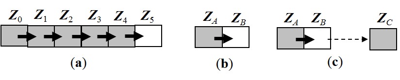
Figure 1. Illustration of 1D Markov chains for spatial data: (a) A 1D Markov chain is a 1D sequence of variables that have the Markovian property. A simulation using a 1D Markov chain model will generate a data sequence based on the Markov transition probability rules. (b) A 1D Markov chain model, with the probability distribution of the state of Z_B depends on the state of Z_A. (c) A 1D Markov chain model with conditioning to a future state (Z_C), presented in Elfeki and Dekking (2001) for constructing the 2D conditional coupled Markov chain model.

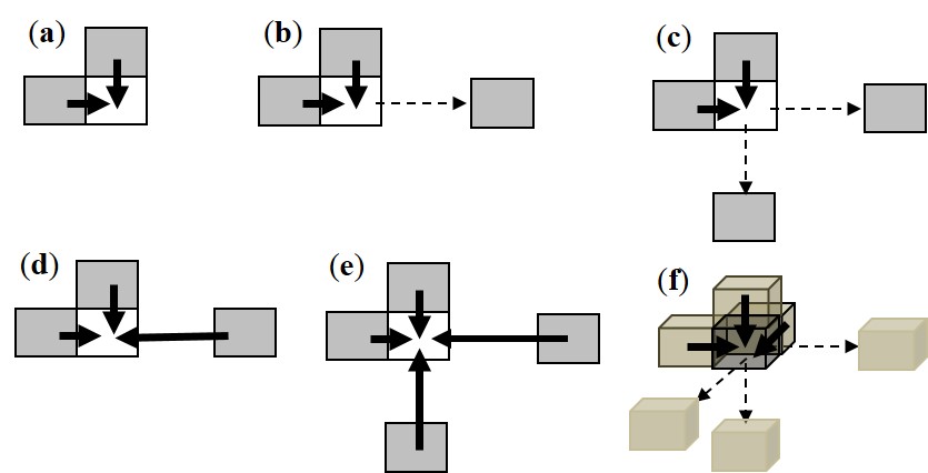
Figure 2. Illustration of 2D and 3D coupled Markov chain (CMC) models: (a) The simplest 2D CMC model for unconditional simulation, presented in Elfeki (1996). (b) The extended 2D CMC model for conditional simulation of subsurface vertical sections, presented in Elfeki and Dekking (2001). (c) The further extended 2D CMC model, used later in horizental 2D simulations with a fixed path (see Li et al. 2004). (d) and (e) 2D tripled and quadrupled Markov chain models, still based on the coupled Markov chain idea (ever tested by us). (f) A 3D CMC model (acutally a 3D tripled Markov chain model), extended from the 2D CMC model (Park et al. 2005). These 2D and 3D models each comprise two or more 1D Markov chains. The 1D Markov chains in these 2D and 3D Markov chain models are assumed to be independent of each other, and their transition probability distributions are multiplied together to form a 2D or 3D model. Because of using two or more 1D Markov chains in each model, conflict transitions occur in all of these models (2D models and further extended 3D model) and have to be excluded. Therefore, all of these 2D and 3D models underestimate small classes if there are small classes in a simulation (a small class means its proportion is lower than the average; and having small classes is the normal situation for categorical fields).

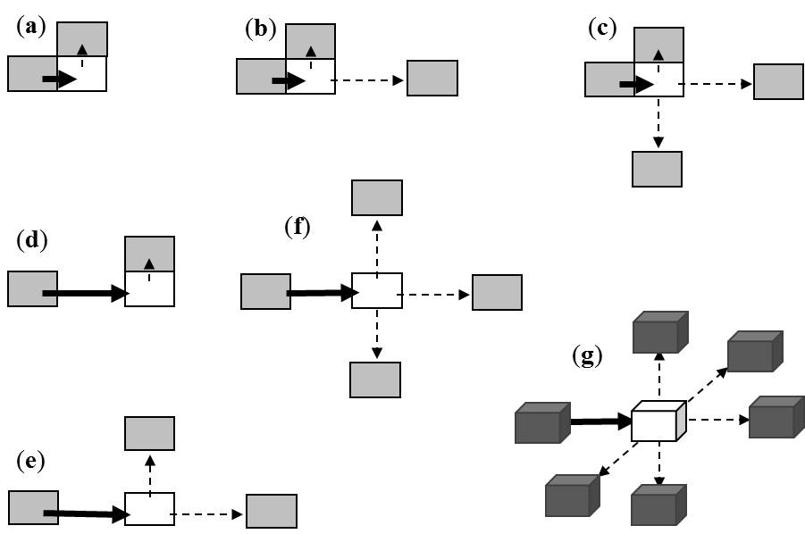
Figure 3. Illustration of specific 2D and 3D Markov chain random field (MCRF) models: (a) and (d) The simplest 2D MCRF models. (b) and (e) The 2D MCRF models, presented in Li and Zhang (2008). (c) and (f) The 2D MCRF models, used in horizontal 2D simulations with fixed paths. (g) The 3D MCRF model, presented in Li (2007, p. 329, eq. (20)). All these models can be drawn from the generalized simplified MCRF model equation in Li (2007) and were presented as MCRF-based spatial Markov chain models. In a 1D space, the MCRF model reduces to a 1D Markov chain model. Outwardly the simplified MCRF models look similar to the CMC models, but essentially they are very different both in model and in surporting theories. First, there is only one Markov chain (the solid arrow) in each of these 2D and 3D models, and other neighborhood data except for the previous state of the Markov chain in each model are all regarded as the data to condition the Markov chain's transition probability distribution. Thus, these models avoid conflict transitions; but they have to be derived using a different way. Second, Bayes' theorem (here spatial sequential Bayesian updating) was used to derive all these spatial models (i.e., the local probability distributions of the MCRFs), and then they were simplified using the spatial conditional independence assumption (which holds here for cardinal-neighbors of a stationary finite Markov field - Pickard random fields) to simplify the multiple-point likelihood terms. Third, some transition probability terms in simplified MCRF models are different. That is why given the same neighborhood the simplified MCRF model and the CMC model generate different results, unless all classes have equal proportions (i.e., no small classes). Therefore, MCRF models do not underestimate small classes. In addition, simplified MCRF models used transiograms for parameter estimation. Note that when we talk "random field", we are meaning the whole finite space to simulate, not just a neighborhood.

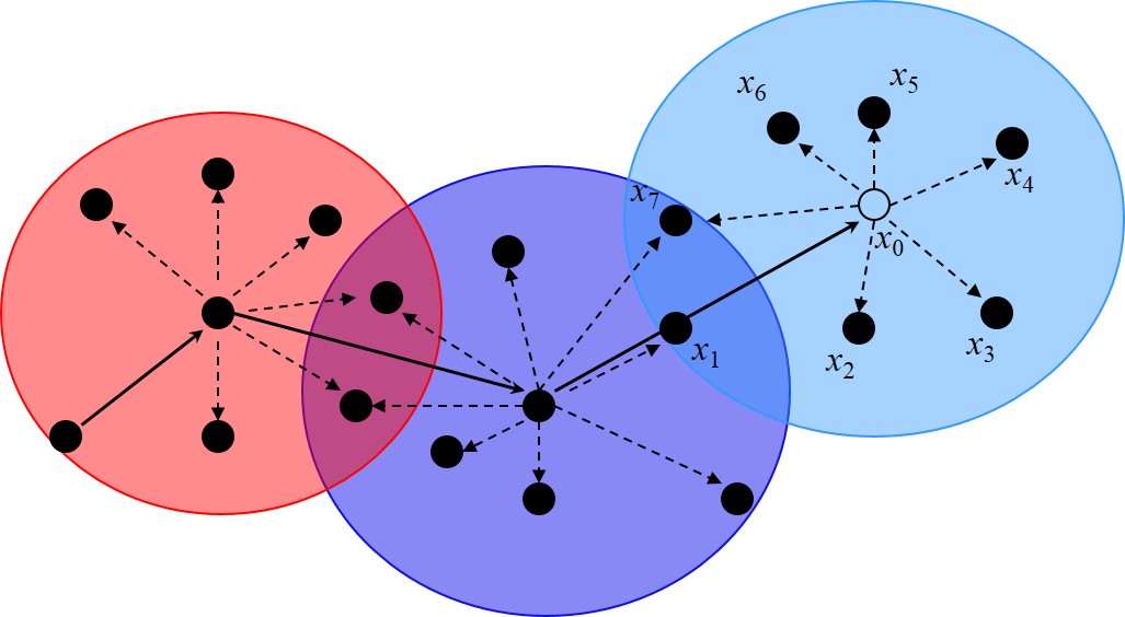
Figure 4. Illustration of the full Markov chain random field (MCRF) model with a random path. A Markov chain (the solid arrow) jumps in a space and at any unobserved location its probability distribution is updated by nearest data within a neighborhood, and the state of the unobserved location is simulated using the updated local probability distribution. This figure was presented in Li (2007). Note that this generalized MCRF model is not limited to 2D. It includes 3D, as given in Li (2007, p. 329, eq. (20)). In addition, it includes the situation that the last visited location of the Markov chain is not within the neighborhood. Also note that in this figure we did not draw the interaction lines between nearest data in each neighborhood although they exist. Similarly, the MCRF model (i.e., the generalized local probability distribution) has to be simplified by using the spatial conditional independence assumption of nearest data to simplify multiple-point likelihood terms if one wants to implement it with only two-point statistics.

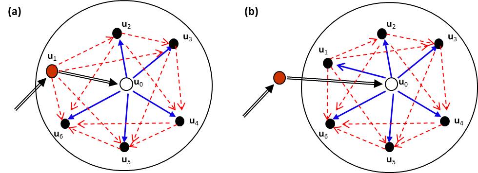
Figure 5. Illustration of the detailed data interactions in the full Markov chain random field (MCRF) model. This figure was presented in Li et al. (2013, 2015). Note that in this figure we show two situations, but the models are the same mathematically, and the difference is that they consider different priors from the Bayesian perspective. This figure provides a clearer and more detailed illustration to the full MCRF model with multi-point likelihoods.

Many years (more than 10 years) have passed since the proposition of the MCRF theory/model. Looking back on this research, we can see that there are some theoretical or methodological breakthroughs in spatial thinking in the transition process from the coupled Markov chain (CMC) theory/model to the Markov chain random field (MCRF) theory/model. These breakthroughs for spatial data analysis and modeling do not involve complex statistical or mathematical knowledge. We do not claim expertise or authority in nonspatial statistics or mathematics. The reasons we could make such breakthroughs are that we encountered the related scientific issues in our study, we explored them for a long time, we developed computer programs by ourselves in each step, and we based our judgments and conclusions on extensive data testing. In addition, we have worked on geostatistical application for a long time (since the beginning of 1990s) and our knowledge in conventional geostatistics was also helpful to us in multidimensional Markov chain modeling and making the breakthroughs. It is these breakthroughs that make the MCRF model not only theoretically sound but also practical. Major breakthroughs may include the followings:
      (1) We considered a locally-conditioned single Markov chain rather than two or more 1D Markov chains in a multi-D Markov chain model, and regarded all other neighborhood data as the data to condition the Markov chain. Thus, the MCRF model avoided conflict transitions, but had to be derived using a different way.
      (2) We used Bayes' theorem to deal with the neighborhood nearest data in the local probability distribution function, and decompose the local probability function to each nearest datum in a neighborhood, thus constructing a local sequential Bayesian updating process for estimating the posterior local probability distribution.
      (3) We extended the cardinal-neighbor conditional independence property of Pickard random fields to sparse data situation and further generalized it for practical use with irregular sample data.
      (4) We used the spatial conditional independence assumption for spatial sample data within a neighborhoood to simplify the full MCRF model into the simplified MCRF model so that the posterior local probability distribution can be estimated using only two-point transition probabilities (fetched from transiogram models).
      (5) We used the spatial conditional independence property of nearest data in cardinal directions in an underlying Pickard random field to rationalize our neighborhood choices for MCRF simulation algorithm design (e.g., the quadrantal neighborhood).
      (6) Following the variogram theory and based on the properties of transition probabilities, the conventional 1D Markov chain theory, and related pioneer studies, we suggested the transiogram concept system and methodology (we proposed two practical joint modeling methods and some math models) to estimate transition probabilities from sample data for implementing simplified MCRF models (note that due to the different requirements of kriging and MCRF to parameters, the transiogram models and joint modeling methods for MCRF simulation may not be all applicable to indicator kriging equation system in computation).

With many years of effort, the MCRF theory/model has been gradually developed into a nonlinear geostatistical approach for simulating categorical fields.

From above illustrations and introductions, one can see that the CMC model was scientifically contributive to the proposition of the MCRF theory/model, despite some misunderstandings that arose among some people who were not familiar with but paid attention to this research topic. Besides being interesting, a major contribution of the CMC model to the MCRF approach (i.e., Markov chain geostatistics) is its defects, which motivated us to explore the possible solutions. It was in this process that we thought of some ideas, captured them, rationalized them theoretically, and tested them to prove their practicality, step by step. One can see that the MCRF theory/model is theoretically complete and rigorous, and methodologically practical. The major breakthroughs in spatial thinking and statistics made in the MCRF approach should be (actually have been) scientifically an important contribution to geo/spatial-statistics and spatial data analysis.

References:

Elfeki, A.M. 1996. Stochastic characterization of geological heterogeneity and its impact on groundwater contaminant transport. Ph.D. diss. Delft University of Technology.

Elfeki, A.M., Dekking, F.M. 2001. A Markov chain model for subsurface characterization: Theory and applications. Math. Geol., 33:569-589.

Li, W. 2007. Markov chain random fields for estimation of categorical variables. Math. Geol., 39(3): 321-335.

Li, W., Zhang, C. 2008. A single-chain-based multidimensional Markov chain model for subsurface characterization. Environ Ecol Stat 15(2): 157-174.

Li, W., Zhang, C., Dey, D.K., Willig, M.R. 2013. Updating categorical soil maps using limited survey data by Bayesian Markov chain cosimulation. Sci World J. Article ID 587284. doi:10.1155/2013/587284.

Li, W., Zhang, C., Willig, M.R., Dey, D.K., Wang, G., You, L. 2015. Bayesian Markov chain random field cosimulation for improving land cover classification accuracy with uncertainty assessment. Math. Geosci., 47(2): 123-148. doi: 10.1007/s11004-014-9553-y.

Li, W. et al. 2004. Two-dimensional Markov chain simulation of soil type spatial distribution. Soil Sci. Soc. Am. J., 68: 1479-1490.

Park, E., Elfeki, A.M.M., Dekking, M. 2005. Characterization of subsurface heterogeneity: Integration of soft and hard information using multidimensional coupled Markov chain approach. p. 193-202. In: C.F. Tsang and J.A. Apps (ed.) Underground injection science and technology. Dev. Water Sci. 52. Elsevier, Amsterdam.

Go Back