Go Back
Simulation algorithms
In the MCRF approach, all stochastic simulation algorithms adopted “sequential simulation”. Sequential simulation means that in a simulation process previously simulated data are all added into the data sequence so that later simulations at unobserved locations are conditioned on previously simulated values. However, the simulation paths and neighborhood structures may be different for different specific simulation algorithms. Random path or partially-random path is preferred in many situations, especially when dealing with irregularly distributed sample data. The major simulation algorithms in classical geostatistics (Goovaerts 1997) all adopted “random-path sequential simulation”.
In multi-dimensional Markov chain modeling, earlier models usually used fixed-paths. Markov mesh models normally used fixed-paths. However, sometimes fixed-paths may result in inclined simulation patterns due to dirrectional correlations induced by asymmetric paths and neighborhoods. So far we have used both random-path and fixed-paths for MCRF sequential simulations. The random-path algorithm we developed uses a random number generator to generate a series of random numbers for selecting the locations to be simulated and the values from local cumulative probability distributions, and once a variable at an unobserved location is simulated its value is added into the conditioning data set. Therefore, its simulaton procedure is the same as the procedure for sequential indicator simulation, except that the models used for estimating local proability distributions are different. We developed two workable fixed-path algorithms - one is the alternate advancing (AA) path and the other is the middle insertation (MI) path, during the efforts to deal with the deficiencies of an earlier impractical two-dimensional Markov chain model. These two paths do not cause pattern inclination because they are symmetric (or quasi-symmetric) in the lateral direction and thus do not induce directional correlation. The AA path was later found to be identical to the herringbone path suggested by Sharp and Aroian (1985) for a unilateral two-dimensional ARMA (autoregressive movingg-average) process model. These two fixed-path algorithms were only used to regular sample data. When sample data are irregularly distributed, the fixed-paths may be used only after the sample data are first connected to make a network by simulation. Because the sample connecting process for making a network from irregularly distributed sample data is complex in computation (Li 2007b), we did not fully implement it. The rationale of the AA path algorithm for modifying an existing impractical two-dimensional Markov chain model has been explained in another page. The MI path algorithm was introduced in Li and Zhang (2007b, 2008) and mentioned in an earlier paper. So in this page we mainly introduce the random-path simulation algorithm (mainly the quadrantal neighborhood for a simplified MCRF model).
It should be mentioned that the MCRF approach is not limitted to 2D models. The general solutions are applicable to any dimensional spaces including 1D to 3D. A specific simplified 3D MCRF model for six nearest neighbors in six cardinal directions was provided in Li (2007a), which can be implemented by using fixed-path and random-path algorithms. Further extension for cosimulation has been done (Li et al. 2013), and further extension for spatiotemporal simulations is also underway.
The quadrantal neighborhood for random-path sequential simulation
The simplified general solutions of MCRFs do not consider the effects of data clusters and data deviation from conditional independence. Apparently, clustered nearest neighbors deviate more from conditional independence than do non-clustered nearest neighbors, and nearest neighbors above the number of cardinal directions deviate more from conditional independence than do nearest neighbors at or below the number of cardinal directions. These situations may affect the estimation of local conditional probability functions. Consequently, dealing with these issues with simplified MCRF models may be necessary in neighborhood and algorithm design or by adding adjustive parameters. These are still within the framework of Markov chain geostatistics or the MCRF appoach.
In real applications, it is unnecessary to consider many nearest known neighbors in different directions. For those nearest known neighbors outside correlation ranges and those approximately located in the same directions with small separate angles but not the closest to the uninformed location u0 being estimated, they can be canceled in simplified MCRF models. Thus, m can be much smaller than the real number of nearest known neighbors in different directions within a search area.
An effective method for avoiding clustered data in a neighborhood is sectorization, which divides a search circle or ellipse into a number of sectors. The conditional independence assumption can hold for adjacent data in cardinal directions given the state of the central location in Pickard random fields (Pickard 1980; Rosholm 1997). Li (2007a) found that such a property may be applied to sparse data situation. Therefore, Li and Zhang (2007a) suggested a random-path MCRF algorithm with a quadrantal neighborhood for sequential simulations conditioned on point sample data, considering that there are actually four cardinal directions for a discretized field to simulate in a Cartesian coordinate system. This sequential simulation algorithm relaxes the cardinal directions to quadrants, by considering four nearest neighbors, one per quadrant, in a search area for estimating the local conditional probability distribution. The simplified MCRF model for this neighborhood is
(1) 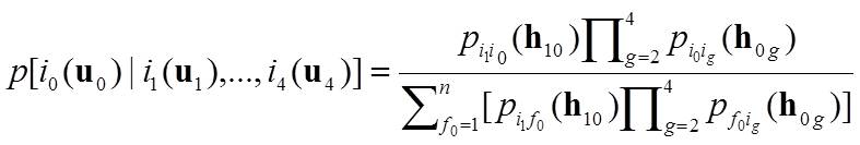 .
.
In this model, it is assumed that the last visited location of the spatial Markov chain is always within the four nearest neighbors; if it is not, we assume the spatial Markov chain comes through one of them. Equation (1) assumes conditional independence of the four nearest neighbors in the four quadrants. Of course, this is not true but just an assumption. However, this neighborhood normally has less deviation from the true conditional independence compared with the neighborhoods without sectorization or with more than four sectors.
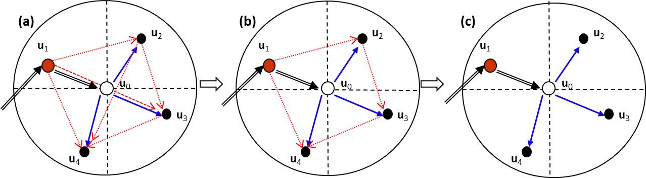
In Figure 1a, we show that the data interactions among four nearest neighbors and the random variable being estimated confirms to a full Bayesian network without simplification, although there is no causality among the data points. So the corresponding probability model involves two-point to five-point statistics. That is why we say that MCRF models are essentially multiple-point statistics. Figure 1b is a partially simplified version of Figure 1a. The corresponding probability model involves two-point to four-point statistics. The completely simplified version (Figure 1c) involves only two-point statistics - transition probability, and the corresponding probabibity model is Equation (1).
There may be no data in some quadrants within a search range at boundaries, or at the beginning of a simulation when sample data are very sparse or a small search radius is used; thus the size of the neighborhood may occasionally be less than four. Equation (1) can adapt to this situation. In case no data can be found in the entire search circle, it is assumed that the spatial Markov chain comes from a location outside the search range. This algorithm was found to be effective in stochastic simulations of categorical fields and superior to indicator kriging based sequential indicator simulation algorithm (Li and Zhang 2007a).
This random-path MCRF simulation algorithm (with Fortran code) was developed during Winter 2005 to Spring 2006. It was initially planned to collaborate with others. Our manuscript was prepared in Spring 2006 and was not planned to submit for publication immediately, because we hoped to submit a proposal with related content for funding application. However, we had to submit it in April 2006, and it was accepted for publication by SSSAJ in August 2006 and was formally published in 2007.
The quadrantal neighborhood can be simply extended to three dimensions (e.g., using cubic lattice).
Other neighborhoods for random-path sequential simulation
Although we have been using the quadrantal neighhorhood due to its rationality, this does not mean that other neighborhoods do not work for random-path sequential simulation. Spatial statisticans such as Ripley (1990) suggested that the conditional independence assumption might be applied to spatial data in a pairwise interaction process. In fact, it is spatial statisticans in statistics who first recognized the Markov chain randon field (MCRF) approach during 2005 to 2006 and supported the publication of our major papers (published in 2007 to 2008). The reason that we did not prefer other neighbrohoods was because we found that neighborhoods wihout consideration of nearest data directions were generally inferior. To clarify some misunderstandings to the MCRF approach (including misuse of some MCRF algorithms), especially the MCRF sequential simulation algorithm, we made a more thorough study to test the performances of MCRF sequential simulation with different neighborhood sizes and structures for the simplified MCRF general model under the conditional independence assumption. The purposes are to: (1) explore whether or not there may be other better neighborhoods, and (2) understand how the model deviation from conditional indepdence impacts simulated results. We tested nine sizes of neighborhoods without sectorization (i.e., size 1 to 9). The results demonstrated that: (1) the quadrantal neighborhood is generally the best choice, and (2) for non-sectored neighborhoods, neighborhood sizes arround 4 (e.g. 3 to 5) performed better than others. See page " Optimal neighborhood structure" for some of the results and explanation. This more thorough work was conducted in 2014. Our paper about this work has not been published.
The middle insertation algorithm for fixed-path sequential simulation
Here we show how the middle insertion (MI) path is used in MCRF simulation of two-dimensional vertical sections of subsurface facies (Li and Zhang 2007b). Of course, it also can be used as a fixed path for horizontal 2D simulation, just like how the AA path was used. Because the MI path is basically symmetric in the lateral direction, it does not induce directional correlation and consequentialy does generate directional artifact. But the boundaries of simulated patches by fixed paths usually are not smooth. These fixed paths were initially developed during 2002 to 2003, mainly for dealing with the pattern inclination problem of the CMC model, but they can be used to the MCRF approach by replacing the CMC model (or the CMC-based TMC model) with the MCRF model with corresponding neighborhood structures. Note that simulation paths themselves are not spatial statistical models, but can impact the exact model forms, choices of neighborhood structures, and simulated patterns. Also note that the CMC model of Elfeki and Dekking (2001) was not a generalized model for spatial data; it was a specific model form fitting a fixed path and neighborhood structure.
The following MCRF model with a MI simulation path corrects the coupled Markov chain model for subsurface characterization, because it is laterally symmetric and does not have conflict transitions due to the use of a single Markov chain. For shallow subsurface characterization, the informed data available for estimating an unobserved location come from three directions – left, right and upper. With a fixed-path, the Markov chain model for subsurface characterization needs to consider three nearest known neighbors in three cardinal directions - left, upper and right (Figure 2a). Assuming the Markov chain jumps from location u1 to the current unobserved location u, and its three nearest neighbors in three cardinal directions are u1, u2, and u3 in the left, up and right directions, respectively, the conditional probability distribution of the Markov chain (i.e., the random variable) at location u can be generally given as
(2) 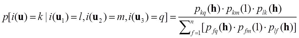 .
.
where n is the number of faceis (or layer types), and h is the distance from the current unobserved location to either of its two nearest known neighbors in a lattice row (Li and Zhang 2007b). Note that in case the number of cells (or pixels) between two nearest known cells in a row is even, we make h1 = h3±1 (i.e., h is not absolutely equal for the left and right nearest neighbors). Such a small lag difference does not influence the lateral symmetry in a simulation that involves many cells in each row between two neighboring boreholes.
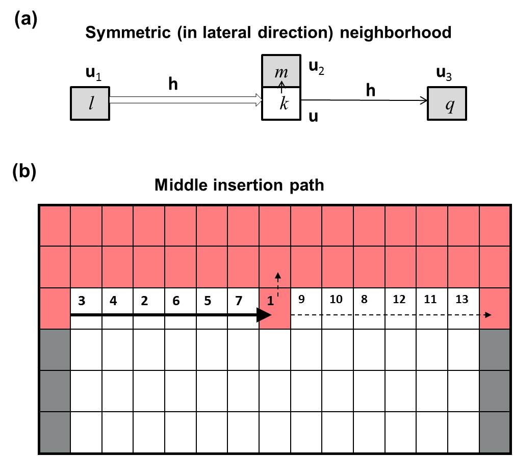
In this MI path algorithm, unobserved locations (cells) in each lattice row are simulated recursuvely by choosing the middle cell between two nearest data cells from left to right (Figure 2b). Because the nearest neighbors are all located in cardinal directions, the conditional independence assumption of nearest neighbors should hold for a stationary special Markov random field. Of course, for real data, interaction between the datum at u2 and the datum at u1 (or at u3) may still exist, and even the Markov property may not hold. In fact, this is just a simple Markov chain model. Because it does not consider the (simulated and obsevred) data in non-cardinal directions, it cannot effectively capture natural curvilinear features. However, including data in non-cardinal directions in the MI or AA fixed-path simulation algorithm may not be proper for simplified MCRF models based on conditional independence assumption due to the strong dependency of nearest data.
References:
Goovaerts P (1997) Geostatistics for natural resources evaluation. Oxford university press, New York.
Li W (2007a) Markov chain random fields for estimation of categorical variables. Math Geol 39: 321–335.
Li W (2007b) A fixed-path Markov chain algorithm for conditional simulation of discrete spatial variables. Math geol 39(2): 159-176.
Li W, Zhang C (2007a) A random-path Markov chain algorithm for simulating categorical soil variables from random point samples. Soil Sci Soc Am J 71(3): 656-668.
Li W, Zhang C (2007b) A middle-insertion algorithm for Markov chain simulation of soil layering. In: Proceedings of the 15th annual ACM international symposium on Advances in geographic information systems (p. 45). ACM., Nov. 7-9, 2007, Seattle, USA. pp. 328-331.
Ripley BD (1990) Gibbsian interaction models. In: Griffith, D.A., ed., Spatial statistics: Past, present, and future: Institute of Mathematical Geography, Syracuse University, p. 3–25.
Li W, Zhang C, Dey DK, Willig MR (2013) Updating categorical soil maps using limited survey data by Bayesian Markov chain cosimulation. Sci World J. Article ID 587284. doi:10.1155/2013/587284.
Li W, Zhang C, Willig MR, Dey DK, Wang G, You L. 2015. Bayesian Markov chain random field cosimulation for improving land cover classification accuracy with uncertainty assessment. Mathematical Geosciences, 47(2): 123-148. doi: 10.1007/s11004-014-9553-y.
Pickard DK (1980) Unilateral Markov fields. Advances in Applied Probability 12(3): 655–671.
Rosholm A (1997) Statistical methods for segmentation and classification of images. Ph.D. dissertation, Technical University of Denmark, Lyngby.
Sharp WE, Aroian LA (1985) The generation of multidimensional autoregressive series by the herringbone method. Math Geol 17: 67–79.