Markov chain geostatistics

Go Back

Optimal neighborhood structure

To approximately meet the requirement of conditional independence of nearest data within a neighborhood, the MCRF sequential simulation (MCSS) algorithm has been using a “quadrantal” (i.e. one nearest datum per quadrant) neighborhood (Li and Zhang 2007). The rationality behind this quadrantal neighborhood idea is one of the properties of Pickard random fields (Pickard 1980) – given the state of the central cell the adjacent neighbors in cardinal directions on a rectangular lattice are conditionally independent. A more detailed description of Pickard random fields and their properties can be found in Rosholm (1997). Such a property of Pickard random fields was extended to sparse spatial data (Li 2007, Li and Zhang 2008). For a real data set, this property for nearest neighbors in cardinal directions becomes an assumption that may approximately hold, or at least does not deviate too much from the truth. In addition, neighborhood sectorization (mainly quadrant/octant search neighborhoods) has been a strategy used in spatial statistics for reducing the effect of data clusters (Arik 1990; Goovaerts 1997). The MCRF approach has no limitation on neighborhood choice due to the generality of the MCRF theory (Li 2007, Li et al. 2015). Neighborhoods other than the quadrantal one (i.e., those neighborhoods without sectorization or with other sector numbers) may be feasible under the conditional independence assumption of nearest data within a neighborhood, although they may deviate more from the conditional independence of nearest neighbors - apparently larger neighborhoods deviate more from the conditional independence of nearest neighbors compared to the quadrantal neighborhood structure, and additionally, smaller neighobrhoods utilize nearest data less sufficiently.

The conditional independence assumption is a typical practical assumption, widely used in statistical methods for non-spatial data, especially in Bayesian analysis, for reducing the complexity of relationships, models and computation (Dawid 1979). Often, even if the assumption obviously does not hold for real data, the simplified models may still work practically and generate useful results. Ripley (1990) suggested that the conditional independence assumption might be applied to spatial data in a pairwise interaction process. Apparently the simplified MCRF models with non-sectored or non-quadrantal neighborhood designs may still work practically in sequential simulations under some conditions, for example, where sample data are approximately randomly or regularly distributed and a random path is used (these can avoid causing strong asymmetry of nearest neighbors in a neighborhood), as suggested in Li (2007).

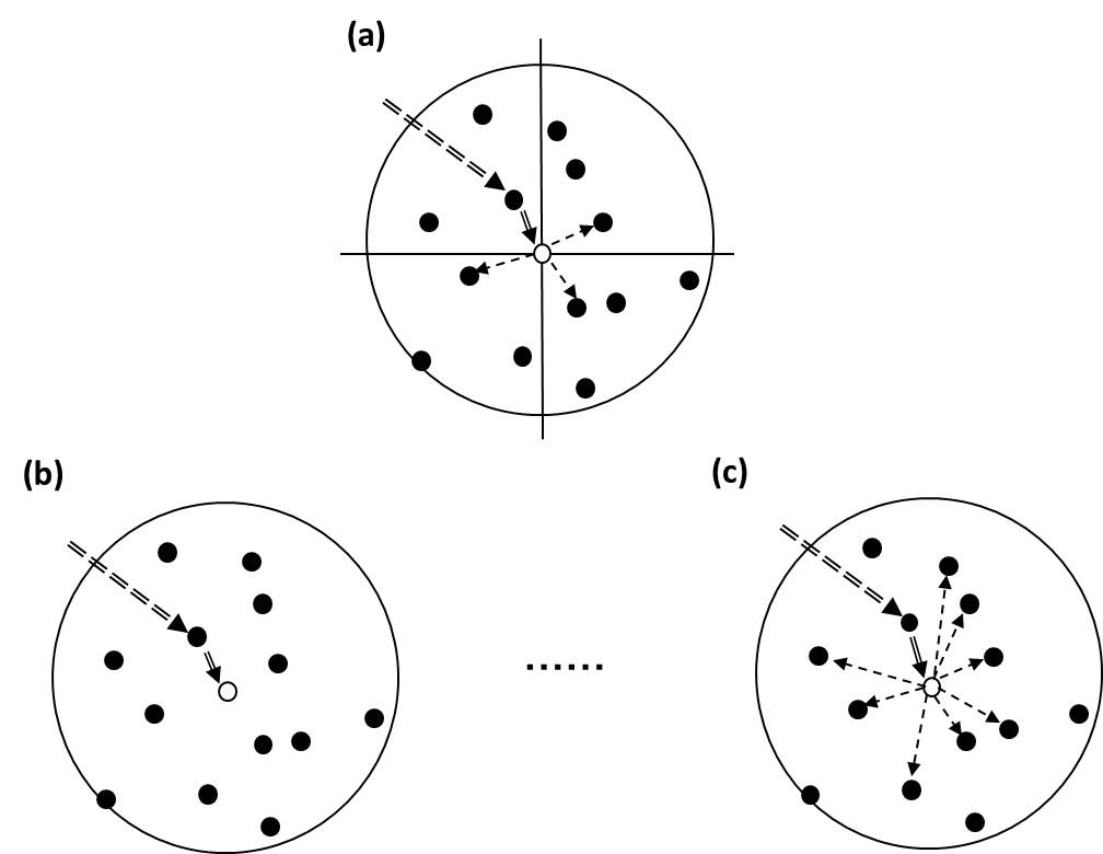
We tested a series of sectored and non-sectored neighborhoods (e.g., nearest-neighbor sizes 1 to 9) and compared them with the quadrantal neighborhood (Figure 1). Part of our result (Figure 2) showed that: (i) neighborhood sizes have obvious impacts on simulation accuracies; (ii) the quadrantal neighborhood is the best choice, performing better than non-sectored neighborhoods and other sectored neighborhoods in both simulation accuracy and pattern rationality. For non-sectored neighborhoods: (a) 3 to 5 nearest data are usually suitable choices (still, 4 is usually the best); Only when sample data are extremely sparse, relatively larger neighborhoods (e.g., 5 or 6) may be a suitable choice for generating more accurate realizations, but their optimal prediction maps have lower accuracies; and (b) while smaller neighborhood sizes (sizes 1 and 2) cause pattern fragmentation, larger neighborhood sizes (usually larger than size 5) may simplify simulated patterns.

Figure 1. Non-sectored MCRF neighborhoods with different neighborhood sizes and the quadrantal MCRF neighborhood under the conditional independence assumption of nearest data. (a): The quadrantal neighborhood. (b) to (c): Non-sectored neighborhoods, considering one to nine nearest neighbors, respectively. The circle represents the search area (i.e., moving window) for seeking nearest neighbors used to estimate the uninformed central point. Black solid dots represent informed data (sample data or previously simulated data).

Figure 2. Simulation accuracies of a multi-class categorical field by the MCRF approach using different non-sectored neighborhoods (1 to 9 nearest neighbors) and the quadrantal neighborhood (4 sectors, with one nearest neighbor from each sector). Accuracies for simulated realizations are averaged from 100 realizations for each simulation case. The original map is used for validation

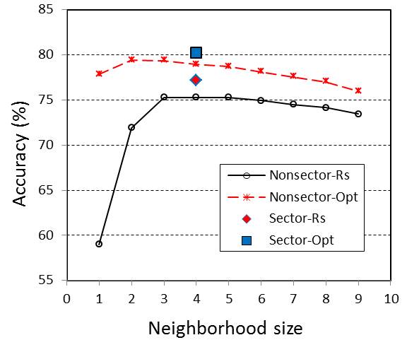
Based on the simulation accuracy data and patterns of the simulated realization maps in our testing simulation cases, we conclude that: (i) departure from conditional independence of nearest data should be the major reason for larger neighborhood sizes (usually larger than 5) to perform worse than medium neighborhood sizes (sizes 3 to 5) under normal sample densities; (ii) approximately meeting the requirement for conditional independence of nearest data (or having less departure from conditional independence) while effectively utilizing nearest data should be the major reason for the quadrantal neighborhood to outperform other neighborhoods; no doubt the quadrantal neighborhood also effectively reduces the effect of data clusters. In general, the quadrantal neighborhood is generally the best choice, as was expected at the beginning based on the rationality of the neighborhood structure which has the least departure from conditional independence.

This systematic testing research was done in 2014 (earlier testing was not systematic). The detailed results were presented in Li and Zhang (2018).

References:

Arik, A. 1990. Effects of search parameters on kriged reserve estimates. Inter J Mining Geol Engineer 8(4): 305-318.

Dawid, A.P. 1979. Conditional independence in statistical theory. J Roy Stat Soc Ser B 41(1): 1-31.

Goovaerts, P. 1997. Geostatistics for natural resources evaluation. Oxford university press.

Li, W. 2007. Markov chain random fields for estimation of categorical variables. Math Geol 39: 321–335.

Li, W., Zhang, C. 2007. A random-path Markov chain algorithm for simulating categorical soil variables from random point samples. Soil Sci Soc Am J 71(3): 656-668.

Li, W., Zhang, C. 2008. A single-chain-based multidimensional Markov chain model for subsurface characterization. Environ Ecol Statist 15(2): 157-174.

Li, W., Zhang, C., Willig, M.R., Dey, D.K., Wang, G., You, L. 2015. Bayesian Markov chain random field cosimulation for improving land cover classification accuracy. Math Geosci 47(2): 123-148.

Li, W., Zhang, C. 2018. Markov chain random fields, spatial Bayesian networks, and optimal neighborhoods for simulation of categorical fields. arXiv preprint arXiv:1807.06111.

Pickard, D.K. 1980. Unilateral Markov fields. Adv Appl Probab 12: 655–671.

Ripley, B.D. 1990. Gibbsian interaction models. In: Griffith, D.A. (ed.) Spatial Statistics: Past, Present, and Future. Institute of Mathematical Geography. p. 3–25.

Rosholm, A. 1997. Statistical Methods for Segmentation and Classification of Images. Ph.D. dissertation, Technical University of Denmark, Lyngby.