Go Back
The Pattern Inclination Problem
Layer/Parcel inclination (also called directional artifact or pattern inclination) is an irrational feature or artifact that appeared in simulated realization maps generated by spatial models with asymmetric neighborhoods and asymmetric simulation paths. This problem was met by us in two-dimensional simulations of soil types and layers using the coupled Markov chain (CMC) model (see W. Li's postdoc report prepared in June 1999 at University of Leuven. The content of this report was presented two times at University of Leuven, Belgium, in Summer 1999). The CMC model was initially suggested by Elfeki in his PhD dissertation in 1996 (the model was not effectively tested, because the dissertation was mainly focused on modeling solute transport in geological structures, and only devoted one chaper to the model. It only simulated one large-scale naturally inclined geological structure without data analysis on multiple simulated realizations). A partner at Leuven thought the model should work well with soil structures, provided the dissertation to me, and suggested me to use the model to simulate soil types. So I developed computer code based on the model described in the dissertation, and made some simulations on soil type and layer spatial distributions (our initial purpose was to study the effect of the spatial variation of soil structures on soil water). The model assumed two 1D Markov chains, one vertical and one lateral, to be independent and coupled (multiplied) them together, with conflict transitions from the two Markov chains being implicitly excluded. Thus, the model considers two adjacent neighboring cells, one upper cell and one left cell, for estimating the current cell. This means that the model used an asymmetric neighborhood, and it also used a fixed asymmetric forward path. Our test showed that the unconditional Markov chain model (which can condition on two boundaries - the left and uper ones) generated only diagonally inclined patterns for soil structures, which were neither expected nor natural, because the orginal soil structures for parameter estimation and boundary conditioning were not inclined. In addition, we found that small classes tended to be underestimated and minor class usually disapeared in simulated maps by the model. Even though the model had these problems, I still thought it was interesting, because being able to use 1D Markov chains to build a 2D model for spatial simulation was interesting in my eye given my knowledge in 1D Markov chains (I just used 1D Markov chain models for simulating 1D soil textural profiles)
Although the model was extended later into a conditional model by Elfeki and Dekking (2001), which could condition on borehole logs ahead (The idea should be a good progress in 2D Markov chain modeling, compared with earlier studies), the layer/parcel inclination problem was not gone when conditioning data were relatively sparse (relative to the correlation ranges of classes in the lateral direction); such situation was especially clear for relatively short-scale and thick layers (i.e., layers with short correlation ranges in the lateral direction and multiple rows of pixels in the vertical direction) in our simulation cases in soil. They (Elfeki and Dekking 2005; Park et al. 2005) also demonstrated simular problems more clearly later. It should be pointed out that although we did not get good results in soil simulation in 1999 (the simulations were only conditioned on two boundaries), we did not simply think the model had no value or was wrong. It just puzzled me. As I wrote in my postdoc report, there were some issues (inclination tendency, underestimated small classes, and impractical parameter estimation) to solve to make the model practical for use in soil type and layer simulation. However at that time, our understandings to the issues were very limited and could not effectively understand and solve them in a short time. I spent three months to read and explore geostatistical books but did not find a solution (it seemed simple but not so simple). That was one reason why we later made large efforts to attempt to eliminate the deficiencies of the model after I came to USA in 2000 (another reason was that after I explored the literature since 1960s in Markov chain modeling in geology, I found that extending 1-D Markov chains into a muti-D spatial model for simulation had been a long-time but not much successful effort in mathematical geology). All of our efforts aimed to solve existing scientific problems, without any intention to embarrass others by telling truth.
At the beginning, we did not know what caused the inclination artifact. In order to modify the model for simulating the spatial distributions of soil types and layers, we tested a variety of different algorithms and found some algorithms (i.e., paths) could overcome the problem. The reason behind this artifact gradually became clear. Our first paper on 2D Markov chain modeling, Li et al. (2004) has two purposes: While overcoming the parcel/layer inclination problem using an alternate advancing algorithm, it also extended the CMC model for simulating soil types in the horizental two dimensions with synthetic survey line data. Although the small class underestimation problem was not solved, simulated realizations looked not bad when a number of survey lines were conditioned. The small class underestimation problem was specifically analyzed with class proportion data in simulated realizations and discussed in that paper. At the time the paper was accepted for publication, the journal (SSSAJ) associate editor asked me for a digital copy of my postdoc report and passed it to a reviewer who asked for it. Please note that when we began our effort to modify the CMC model in Milwaukee, the paper of Elfeki and Dekking (2001) had not come out. After we knew the paper in 2003, we immediately obtained it from a library, adopted their new idea and recognized their conditional CMC model (At that time many journals had not become avaialble online, and our manuscripts for Math. Geol. were all submitted by mails in and before 2006). But their conditional CMC model still did not solve the layer inclination tendency and small class underestimation tendency problems, which we had been making effort to solve.
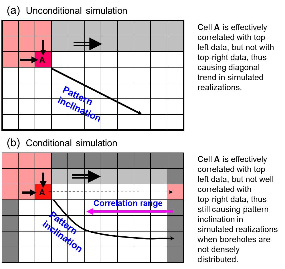
The following Figure 1 shows how layer/parcel inclination is induced in a simulation: With a forward simulation path, the simulated cell A is only correlated with the upper and left cells. If all cells are simulated in this way, each simulated cell will be affected only by the upper-left data and not by upper-right data. In conditional simulation (conditioning on a borehole log ahead), the simulated cell A will not be well-affected by the borehole log ahead when the distance is long (relative to the lateral correlation ranges of classes). Thus, in the final simulated realization maps, each cell will be still well-affected by the upper-left data and not by the upper-right data. This means that the the asymmetric neighborhood, plus an asymmetric simulation path, induces directional correlation among simulated data, consequently causing a pattern with irrational directional artifacts (see Figure 2).
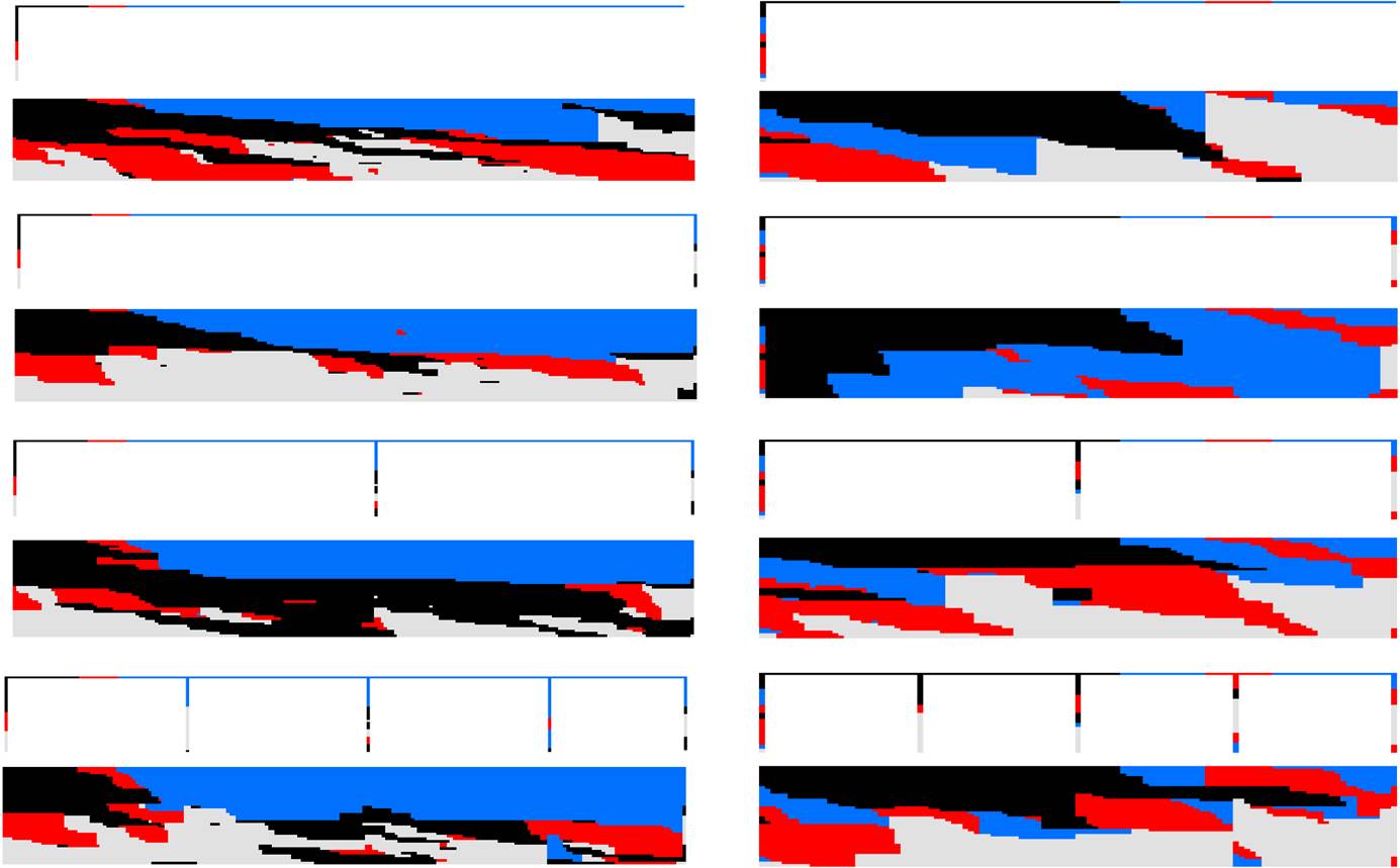
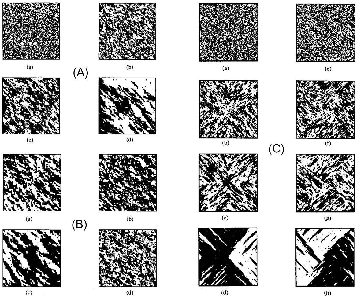
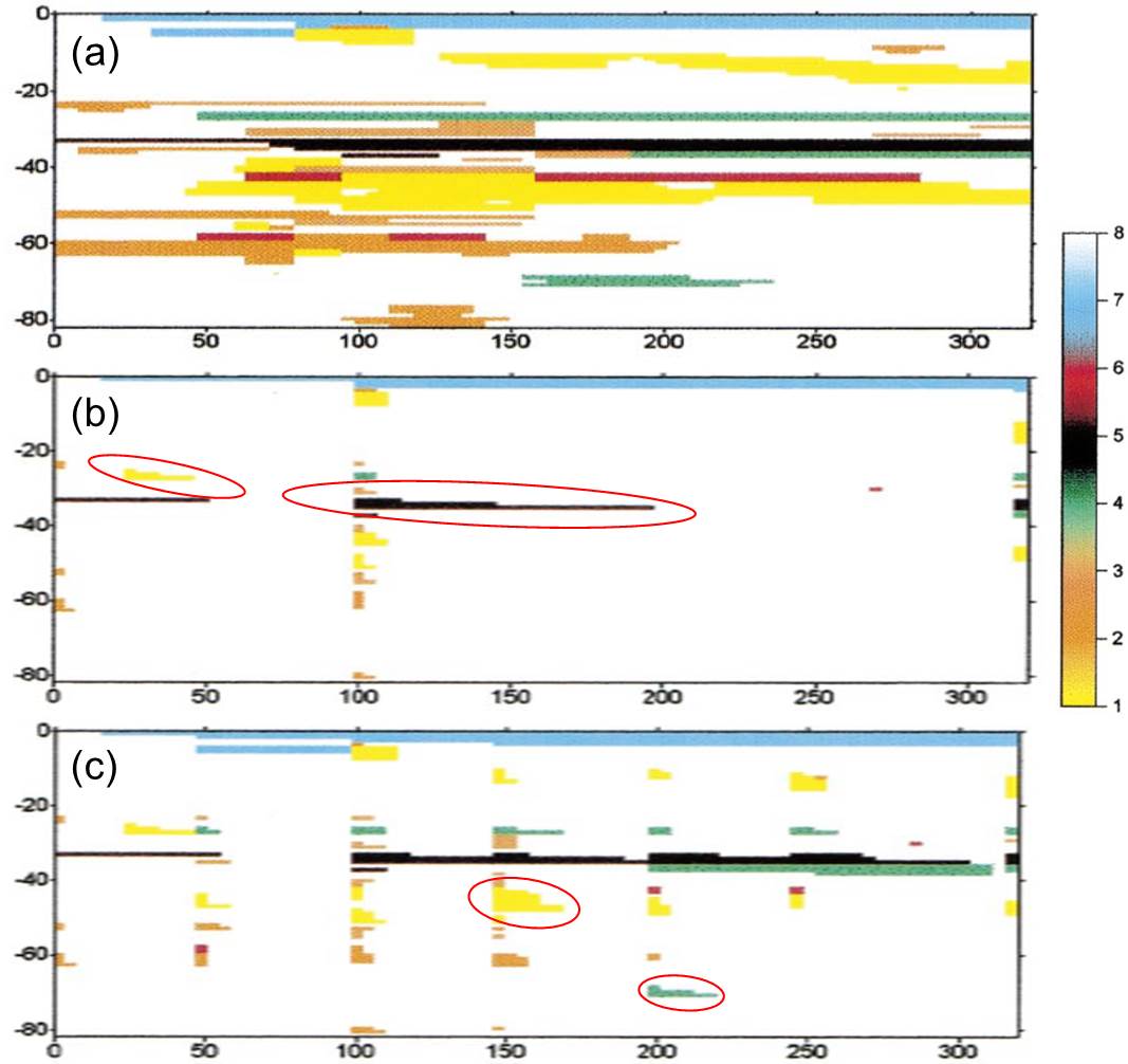
The directional artifact problem - layer inclination - was also shown more clearly later by Elfeki and Dekking (2005) and Park et al. (2005) (see Figure 3), although they did not mention the small class underestimation problem in the paper. Elfeki and Dekking (2005) suggested a forward-backward coupled Markov chain model in the paper. But that model did not truly solve the problem, becuse the model still did not make a symmetric or qusi-symmetric path. While it seemed that they did not care much about the drawbacks of the model, we treated them very seriously and made large efforts because these problems cannot be ignored in categorical soil mapping, where soil patterns are much more complex. The categorical patterns in soils are often very different from those in geology. That might be why we eventually solved the problems. Arguing on whether the defects of the CMC model are clear or not in some special cases is not meaningful, because the tendencies always exist as facts (they were theoretically proved) no matter whether they are clear or not in some special cases.
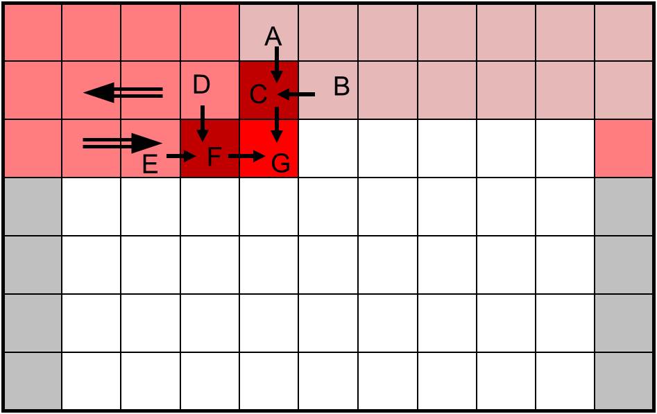
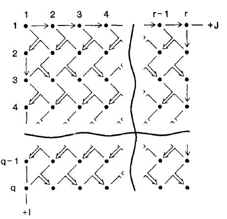
To make the CMC method practical in soil type/layer simulation, this problem had to be solved. So we tested different simulation algorithms (or paths), and found that the alternate-advancing (AA) algorithm and the middle-insertion (MI) algorithm can overcome the problem, although they may not be perfect. The rationality behind these algorithms is that their simulation paths are symmetric (MI path is symmetric) or quasi-symmetric (AA path is quasi-symmetric) in the lateral direction. Thus, the simulated cell will be well correlated with both upper-right and upper-left data, and the pattern inclination problem may be overcome. Figure 4 shows why the currenly simulated cell G is well correlated with already simulated data in both sides in a simulation using the AA path: A and B generate C, so C is correlated with upper-right data; D and E generate F, so F is correlated with upper-left data; C and F generate G, thus G is correlated with data in both sides.
This pattern inclination problem may be regarded as an algorithm problem, that is, a properly designed simulation path or algorithm without changing the basic model idea can solve the problem. But it also can be considered as a model problem, that is, when we change the fixed simulation path, the specific model form (including data correlation) is also changed. For example, the AA path used three Markov chains to form two couplings and let them advance alternately. We said three Markov chains because they use three different transition probability matrices. That is why we called the revised model a triplex Markov chain (TMC) model. The MI path needs to triple three Markov chains together. But after the CMC model was extended and could condition to a “future state”, the MI path also could directly use the CMC model with two multiple-step transition probabilities. Anyway, the exact model form has to be changed with the fixed path change. The essential change behind the fixed-path change is the change in spatial correlation of simlated data (see Figure 3). However, no matter how the model form changes, the basic model idea is the same – coupling (multiplying) two or more 1-D Markov chains together to form a nonlinear simulation model (this is different from a linear additive model). Therefore, our earlier efforts were based on the CMC idea and aimed to make it more practical. Of course, these fixed paths can be directly used in the theoretically more rational single-chain-based multidimensional Markov chain model (i.e., the Markov chain random field (MCRF) model), as proposed later (Li and Zhang, 2007, 2008), because the MCRF model solved another problem of the CMC model - the small class underrepresentation problem, which will be talked separately.
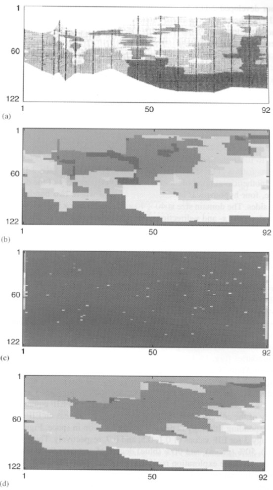
The pattern inclination problem is not unique for the CMC model. We later found that in Markov mesh modeling (Markov mesh models use asymmetric neighborhoods and fixed simulation paths), similar problem may occur if the unilateral neighborhood used is not sufficiently large and it is a known issue in Markov mesh modeling, as demonstrated in Gray et al. (1994). Figure 5 shows some simulated realizations using some Markov mesh models with different simulation algorithms, all from Gray et al. (1994). One can see the pattern inclination (and the windmill) effects. But Gray et al. (1994) did not provide a method to avoid the problem. Note that Markov mesh models were also called Markov chain models or Markov mesh random field models in image analysis.
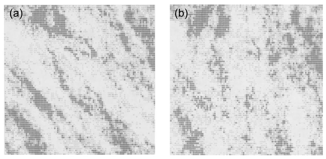
This directional effect problem was also encountered in extending 1-D autoregressive (AR) processes into multiple dimensions, and the herringbone method was proposed to solve the problem (Sharp and Aroian, 1985; Turner and Sharp 1994; Sharp and Turner 1999). Figure 6 shows two realizations, one was generated by a unilateral AR model and the other was generated by the herringbone AR model, both from Sharp and Aroian (1985). Note that here the simulated variable is a continuous spatial variable. The herringbone method suggested alternating the direction of propagation of the process from lattice row to lattice row in the form of a herringbone pattern so that overall isotropy could be induced (see Figure 7). Therefore, the AA path is essentially identical to the herringbone method. Unfortunately, because we did not know the herringbone method at that time (actually this method was not known in the field of Markov chain/mesh modeling), our paper (Li et al. 2004) did not cite the works of Sharp and his coauthors (After knowing that in 2006, our later major papers about the MCRF idea published in 2007 and 2008, which used the AA path, mentioned this point). Therefore, if the AA path still has values, the first proposition of such a fixed-path for spatial simulation should be attributed to Sharp and his coauthors.
In general, using some symmetric or quasi-symmetric paths, the directional effect caused by asymmetric neighborhoods may be avoided. Nevertheless, fixed paths may not be the best choice in many situations. For example, they cannot generate smooth polygon boundaries for simulation of categorical fields. Our explanaion above is intuitive. For theoretical explanation, see papers of Sharp and his coauthors.
It should be noted that the pattern inclination problem may not be always obvious. If the original pattern is naturally inclined along the simulation direction (e.g., from left-top corner to bottom-right corner), it can be approximately generated. If the orginal layers are strongly autocorrelated in the lateral direction (i.e., very long straight layers) (input auto-transition probabilities in the lateral direction are close to 1.0) but much weakly autocorrelated in the vertical direction, their inclination will not be apparent in conditional simulation (but still visible in unconditional simulation; see Figure 10); however, those relatively thick and short layers show clear inclination tendency (see Figures 8 and 9). This kind of patterns may exist in geology, but are very rare in soil structures. That is probably why our previous study with the CMC model and Elfeki's study had different emphases. Of course, if borehole or survey line data are very dense (relative to correlation ranges of classes), any problem may disappear in conditional simulations. However, if sample data are scattered points rather than boreholes or survey lines, the CMC model may not work well unless all classes have similar proportions or sample data are extremely dense. Anyway, no matter whether the problems are obvious or not in some different cases, the defects of the CMC model are proved facts both theoretically and in simulation. There is no need to repeatedly argue and demonstrate, either to show those problems or to show the workability of the CMC model under some special situations. It is really unimaginable that, in order to attack the MCRF model, some people recently even used fake data or wrong input parameters to show that the CMC model could work well. While they were troubling the MCRF approach and its proposers, were they also embarrassing others?
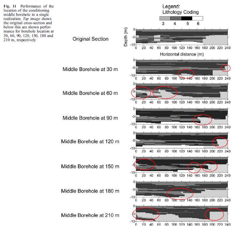
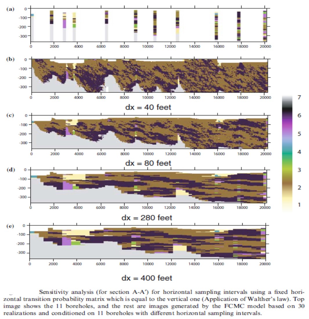
Above Figure 11 is from Park et al. (2005, figure 16.2). Obiously, the authors used an asymmetrical path (the forward path) to conduct the CMC simulation. The simulated realization images clearly show that when the CMC simulation was conditoned on dense well data, layer inclination and small class underestimation were not apparent, but when the simulation was conditioned on only two boundary wells plus some sparse point sample data, both layer inclination and small class underestimation were strong. If a symmetrical or quasi-symmetrical path, such as the AA path and MI path mentioned above, were used, at least the layer inclination problem should have been gone.
References:
[1] Elfeki, A.M. 1996. Stochastic characterization of geological heterogeneity and its impact on groundwater contaminant transport. Ph.D. diss. Delft University of Technology.
[2] Elfeki, A.M., and F.M. Dekking. 2001. A Markov chain model for subsurface characterization: Theory and applications. Math. Geol., 33:569–589.
[3] Elfeki, A.M.M., and F.M. Dekking. 2005. Modelling subsurface heterogeneity by coupled Markov chains: directional dependency, Walther’s law and entropy. Geotech. Geol. Eng., 23(6): 721-756.
[4] Elfeki, A.M.M., and F.M. Dekking. 2007. Reducing geological uncertainty by conditioning on boreholes: The coupled Markov chain approach, Hydrogeol. J., 15, 1439–1455.
[5] Gray, A.J., Kay, I.W., Titterington, D.M., 1994. An empirical study of the simulation of various models used for images. IEEE Trans. Pattern Anal. Mach. Intell., 16(5): 507–513.
[6] Li, W., Zhang, C., Burt, J.E., Zhu, A.X., Feyen, J. 2004. Two-dimensional Markov chain simulation of soil type spatial distribution. Soil Sci. Soc. Am. J., 68: 1479–1490.
[7] Li, W., Zhang, C. 2007. A middle-insertion algorithm for Markov chain simulation of soil layering. Proceedings of ACMGIS 2007, 15th ACM International Symposium on Advances in Geographic Information Systems, Nov. 7-9, 2007, Seattle, USA. p. 328-331.
[8] Li, W., Zhang, C. 2008. A single-chain-based multidimensional Markov chain model for subsurface characterization. Environmental and Ecological Statistics, 15(2): 157-174.
[9] Park, E., Elfeki, A.M.M., Dekking, M. 2005. Characterization of subsurface heterogeneity: Integration of soft and hard information using multidimensional coupled Markov chain approach. p. 193-202. In: C.F. Tsang and J.A. Apps (ed.) Underground injection science and technology. Dev. Water Sci. 52. Elsevier, Amsterdam.
[10] Sharp, W.E., Aroian, L.A. 1985. The generation of multidimensional autoregressive series by the herringbone method. Math. Geol., 17: 67–79.
[11] Sharp, W.E., Turner, B.F., 1999. The extension of a unilateral first-order autoregressive process from a square net to an isometric lattice using the herringbone method. In: Lippard, S.J., Nass, A., Sinding-Larsen, R., eds., Proceedings of IMAG’99, 6–11 August 1999, Trondheim, p. 255–259.
[12] Turner, B.F., Sharp, W.E., 1994. Unilateral ARMA processes on a square net by the herringbone method. Math. Geol., 26(5): 557–564.
[13] Zhang, C., Li, W. 2008. A comparative study of nonlinear Markov chain models in conditional simulation of categorical variables from regular samples. Stoch. Environ. Res. Risk Assess., 22(2): 217-230.