Go Back
Cosimulation models
Similar to cokriging models in classical geostatistics (Matheron 1971; Goovaerts 1998), MCRF cosimulation models (coMCRFs) also can be established through extending the MCRF solution (see Li et al. 2013, 2015). Bayesian philosophy has been used in geostatistics for incorporating soft data since 1980s (e.g. Omre 1987; Woodbury 1989; Christakos 1990; Banerjee et al. 2004). Based on the Bayesian inference principle (Bayes 1763), a coMCRF model may be regarded as the Bayesian update of a MCRF model based on new evidence of auxiliary data. In the MCRF approach, one of our main focuses is the MCRF cosimulation.
Assuming X is a target categorical spatial variable to be estimated and E is an auxiliary data set, the Bayesian inference formula for this knowledge updating can be written as
(1) ![]()
where C is a constant; P(X) represents the local probability distribution of X (here it is the MCRF model or one of its simplified forms), which serves as the prior here; P(E|X) is the probability of observing E given X, that is, the likelihood term to update the prior with new evidence of E. Because a MCRF model is a spatial Bayesian model at the neighborhood level with local sequential Bayesian updating on different nearest data, the incorporation of an auxiliary data set in a Co-MCRF model is essentially a further Bayesian update to a MCRF model. E can be a set of auxiliary variables. For n mutually independent auxiliary variables (i.e., conditionally independent auxiliary variables given X) E = {e1,…,en}, we have
(2) ![]()
Based on above Bayesian principle, we can expand a MCRF model into a Co-MCRF model to incorporate auxiliary variables through cosimulation.
In fact, the contributions of auxiliary variables may be incorporated through different methods. One way is to use the formulation of addition (to some extent similar to cokriging), that is, by including one contribution term for each auxiliary variable. Alternatively, the formulation of multiplication can be used to incorporate auxiliary variables (Li et al. 2013). Below we may regard the data of auxiliary variables as nearest neighbors of the uninformed location u0 in different variable spaces. Thus, the multiplication formulation given in above Equation (2) was used to construct a Co-MCRF model. Considering only the colocated cosimulation case, the Co-MCRF model with k auxiliary variables (Figure 1a) can be written as
(3) ![]()
where r0(k) represents the state of the kth auxiliary variable at the co-location, and qi0r0(l) represents the cross transition probability from class i0 at location u0 in the primary variable space to class r0 at the co-location in the kth auxiliary variable space. The cross transiograms from the primary variable to auxiliary variables reduce to cross transition probabilities due to the co-location property. This kind of cross transition probability (or transiogram) between classes of two different spatial variables is called a cross-field transition probability (or transiogram) (Li et al. 2013). Because the co-located datum of an auxiliary variable is in another variable space, it may be assumed to be conditionally independent of the nearest neighbors of the uninformed location u0 in the primary variable space. The cross-field transition probabilities from the primary variable to each auxiliary variable, however, must be estimated separately. In this equation, the cross correlations between auxiliary variables are not dealt with and they are practically assumed to be independent of each other (i.e., conditionally independent given the primary variable).
If only one auxiliary variable is incorporated, the Co-MCRF model further reduces to
(4) ![]()
This model still can be regarded as a Bayesian inference model. Compared to the MCRF model without incorporating auxiliary variables, this Co-MCRF model uses one more data layer – an auxiliary data set, where each co-located datum may be regarded as new evidence for further updating the local conditional probability distribution.
Above Co-MCRF models are applicable to any dimensional spaces (1D to 3D and spatiotemporal space).
For two-dimensional cosimulation of categorical fields, we may consider using the quadrantal neighborhood due to its rationality. If one auxiliary variable is considered, the two-dimensional Co-MCRF model may be illustrated as Figure 1b.
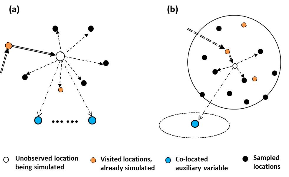
Figure 1. Illustrations of the MCRF co-simulation model with conditional independence assumption (a) and the two-dimensional co-located Co-MCRF model with the quadrantal neighborhood (b) for Markov chain geostatistical co-simulation. Double arrows represent the moving directions of the Markov chain. Dash arrows represent the interactions of the Markov chain with its nearest known neighbors and ancillary data.
As a natural extension of the MCRF model, our coMCRF model and simulation algorithm for remote sensing land cover postclassification and soil map updating were initially developed during 2010 to 2011. They were first presented on GIScience 2012 and GeoComputation 2013, respectively (with extended abstracts published online). However, due to some reasons (e.g. the challenges to the MCRF model reach the first peak in 2011. See our published comment letters in 2012), our manuscript publication on journals had to be repeatedly delayed, and they were finally published in 2013 and 2015 (see Li et al. 2013 and Li et al. 2015. The latter became online in summer 2014). Further testing of the method with large image, complex landscape, and different preclassifiers was done in 2014 (see our paper Zhang et al. 2016), and further improvement of the method for land cover land use postclassification with spectral similarity measures was done in 2015 (see our paper Zhang et al. 2017).
References:
Banerjee S, Carlin BP, Gelfand AE (2004) Hierarchical modeling and analysis for spatial data. CRC Press.
Bayes T (1763) An essay towards solving a problem in the doctrine of chances. Phil Trans Royal Soc London 53: 330-418.
Christakos G (1990) A Bayesian/maximum-entropy view to the spatial estimation problem. Math Geol 22(7): 763-777.
Goovaerts P (1998) Ordinary cokriging revisited. Math Geol 30(1):21–42.
Li W, Zhang C, Dey DK, Willig MR (2013) Updating categorical soil maps using limited survey data by Bayesian Markov chain cosimulation. Sci World J. Article ID 587284. doi:10.1155/2013/587284.
Li W, Zhang C, Willig MR, Dey DK, Wang G, You L (2015) Bayesian Markov chain random field cosimulation for improving land cover classification accuracy. Math Geosci 47(2): 123-148.
Matheron, G (1971) The theory of regionalized variables and its applications. Les Cahiers du Centre de Morphologie Mathematique de Fontainebleau, No. 5
Omre H (1987) Bayesian kriging - Merging observations and qualified guesses in kriging. Math Geol 19(1): 25–39.
Woodbury AD (1989) Bayesian updating revisited. Math Geol 21(3): 285-308
Zhang, W., W. Li and C. Zhang. 2016. Land cover post-classifications by Markov chain geostatistical cosimulation based on pre-classifications by different conventional classifiers. International Journal of Remote Sensing, 37(4): 926-949.
Zhang, W., W. Li, C. Zhang, and X. Li. 2017. Incorporating spectral similarity into Markov chain geostatistical cosimulation for reducing smoothing effect in land cover postclassification. IEEE Journal of Selected Topics in Applied Earth Observations and Remote Sensing, 10(3): 1082-1095.